On the Visualization of Dynamic Structure:
Understanding the distinction between static and dynamic network topology
Kurt A. Richardson & Andrew Tait
Introduction
Understanding the structure of complex networks and uncovering the properties of their constituents has been, for many decades, at the center of study of several fundamental sciences, such as discrete mathematics and graph theory. In the past decade there has been an explosion of interest in complex network data, especially in the fields of biological and social networks. Given the large scale and interconnected nature of these types of networks there is a need for tools (both mathematical and computational) that enable us to make sense of these massive structures.
The field of network theory/analysis has emerged in the last decade or so offering tools that allow analysts to begin to comprehend, and therefore intervene in, complex networks.
Social Network Analysis (SNA) (Borgatti et al., 2013) has grabbed most of the headlines (e.g., Economist, 2015) – in no small part due to the growth of social media. However, SNA focuses primarily on the extraction and analysis of static networks. This precludes any understanding of how networks evolve or how the structure of the network shapes behavior. Dynamic network analysis (DNA) is essential if we wish to gain comprehensive access to the secrets networks hold. A National Academy of Sciences workshop on SNA for building community disaster resilience concluded that “Building resiliency into social networks requires an understanding of the dynamic nature of networks and of how positive changes that prevent network failure during a disaster may be promoted” (Magsino 2009).
“Dynamic network analysis (DNA) is an emergent scientific field that brings together traditional social network analysis (SNA), link analysis (LA), social simulation and multi-agent systems (MAS) within network science and network theory. There are two aspects of this field. The first is the statistical analysis of DNA data. The second is the utilization of simulation to address issues of network dynamics” (https://en.wikipedia.org/wiki/Dynamic_network_analysis). Statistical analysis of static networks is by far the more mature of these two aspects of DNA. In this paper we focus more on the simulation of dynamic networks. In so doing, we illustrate the distinction between static network topology and the actual active network structure that emerges when a dynamic nonlinear network follows a range of different attractors. In this way we illustrate, for a fairly simple Small World network, that when it comes to designing network interventions just seeing who or what is connected to who or what is insufficient to obtain a complete understanding of the network.
This paper will explore network dynamics using a simple Boolean network model. Using this framework, the concepts of information barriers and emergent effective dynamic structure will be explicated. We will also consider the concept of ‘network compressibility’ as an approach to simplifying networks and examine to extent to which it can be applied to Boolean networks. We also present some initial speculations as to how this work might inform the analysis of real-world dynamic networks.
Boolean Network Analysis
As mentioned above, a major limitation of traditional network analysis tools (such as SNA) is that they focus primarily on the static topology (structure) of the network of interest. There is little to no accounting of how information flows around the network and how information is processed by the network nodes. Boolean networks are dynamic, and thus can be used to provide insights into how the flow of information and its transformation impacts the effective (dynamic) network topology.
As a trivial example, imagine a fully inter-connected network where each node is connected, in both directions, to every other node. Additionally, each node transforms incoming information by ignoring it, i.e., the node contains a set of rules whose net result is that none of the incoming information affect the node’s state; the node’s state remains the same regardless of incoming signals. From a conventional network/graph-based analysis, the network would appear to have many hundreds/thousands of feedback loops – such a high level of connectivity itself is of interest. However, from dynamical considerations we would see that this network is really very dull. In the language of nonlinear dynamics theory, this network has many (equal to the number of possible network states, which for a Boolean network is 2N, where N is the number of nodes) point attractors which completely define its qualitative dynamics; basically the network’s state does not change from the initial conditions used to ‘seed’ it -- not very interesting at all. Although this example is trivial, it does highlight in an extreme way how excluding dynamical considerations can lead to very misleading conclusions about the significance of the connectedness of some networks.
It seems self-evident that static networks are going to provide a limited perspective on most social systems. Companies, for instance, are swirling masses of blossoming and decaying relationships (edges).
The aim of this section is to consider how information flows determine effective network structure. We won’t go into much detail here about how a formal Boolean Network is defined. The interested reader is directed to Wikipedia (https://en.wikipedia.org/wiki/Boolean_network). In the opinion of the authors Boolean network analysis provides a relatively simple tool for exploring the fundamental ‘physics’ of complexity theory.
A Boolean network is simply a set of connected nodes. Each node can adopt one of two states: 0 or 1 (hence ‘Boolean’), and has associated with it a rule that relates the next state of the node from the current states of the nodes that are connected to that node. Connections in Boolean networks have direction. If A is connected to B this means that information can flow directly from A to B. It does not follow that information can flow directly from B to A, unless B is also connected to A. This does not exclude the possibility that B is part of a feedback loop that eventually feeds-back to A. Figures 1a and 1b show pictorially the Boolean network that is used throughout this study. The two figures represent the same network, just drawn differently.
For 1b, the nodes were randomly allotted to a point on a simple grid. The total distance between all the nodes was then calculated; literally the length of all the connections was totaled. The nodes were then reallocated and the calculation rerun. This process was repeated 100,000 times, and the layout with the shortest total distance was deemed the most efficient one. This is the layout shown in Figure 1b.
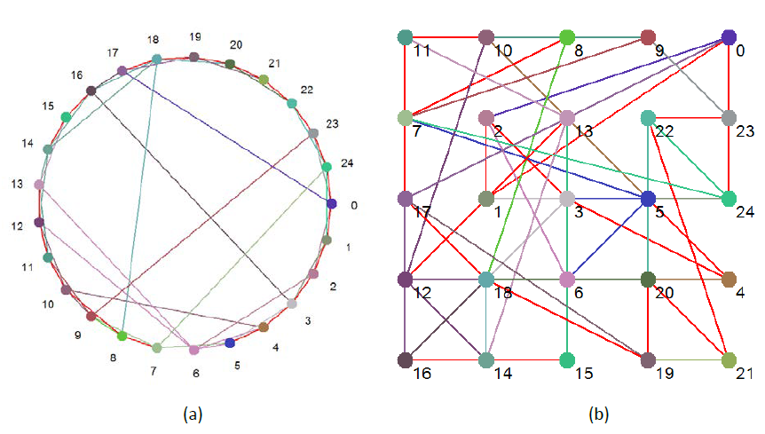
Figure 1 Boolean ‘Small World’ network used for this study
The red connections indicate that the nodes are connected in both directions, otherwise the color of an edge is determined by the color of the node it come out of.
Figure 1 just illustrates the network’s static topology. Table 2 shows the same network in tabular form, but also includes the all-important Boolean rule that is associated with each node, and which is used to process the information (the collection of states) from incoming connections. We can see here that the number of incoming connections to any one node ranges from 1 (Nodes 6, 7, and 14) to 5 (Node 12).
| Node | Rule | Number of Incoming Connections | Incoming Connections | ||||
|---|---|---|---|---|---|---|---|
| 0 | 6A96 | 4 | 24 | 1 | 2 | 23 | |
| 1 | 1E | 3 | 24 | 0 | 2 | ||
| 2 | 5 | 2 | 1 | 3 | |||
| 3 | DE36 | 4 | 1 | 2 | 4 | 16 | |
| 4 | 5A35 | 4 | 3 | 5 | 6 | 10 | |
| 5 | B493 | 4 | 3 | 4 | 6 | 7 | |
| 6 | 2 | 1 | 2 | ||||
| 7 | 2 | 1 | 8 | ||||
| 8 | 5B | 3 | 7 | 10 | 18 | ||
| 9 | A6 | 3 | 7 | 8 | 10 | ||
| 10 | B | 2 | 8 | 11 | |||
| 11 | F0 | 3 | 9 | 10 | 12 | ||
| 12 | 54FD75C8 | 5 | 11 | 13 | 14 | 10 | 6 |
| 13 | E6CA | 4 | 11 | 12 | 14 | 6 | |
| 14 | 2 | 1 | 15 | ||||
| 15 | D3 | 3 | 13 | 14 | 16 | ||
| 16 | 38 | 3 | 14 | 15 | 18 | ||
| 17 | 99 | 3 | 16 | 18 | 0 | ||
| 18 | 81 | 3 | 17 | 19 | 14 | ||
| 19 | A6 | 3 | 17 | 18 | 20 | ||
| 20 | 2D | 3 | 18 | 19 | 21 | ||
| 21 | 4D | 3 | 19 | 20 | 22 | ||
| 22 | 23 | 3 | 20 | 21 | 23 | ||
| 23 | 87 | 3 | 22 | 24 | 9 | ||
| 24 | 6B8E | 4 | 22 | 23 | 0 | 7 | |
Table 1 Lists the Boolean rule and set of incoming connections from other nodes for each node in the network
To understand how the Rule determines a node’s next state, let’s consider node 10, which has two inputs (or neighbors – nodes 8 and 11), whose states are combined via the Rule 0xB (hex for 1011 in binary). Table 2 shows how different combinations of the node 10’s inputs are processed:
| Node 8 state | Node 11 state | Resulting Node 10 state |
| 0 | 0 | 1 |
| 0 | 1 | 0 |
| 1 | 0 | 1 |
| 1 | 1 | 1 |
Table 2 Rule table for Node 10. Note that the rows of the third column combined are 1011, or 0xB. This is the Boolean rule for Node 10.
The rule value represents the outputs of a truth table where the inputs are all the possible combinations of the input nodes. The input columns, in this case, are ordered by node number and the rows are ordered according to the binary number that the inputs represent – i.e., 00, 01, 10, 11.
Network Structure
Before looking at the dynamics of this network in detail there are number of measurements we can calculate that characterize the network’s static topology. Table 3 list a number of important metrics that characterize this network.
| Number of nodes | 25 |
| Number of edges | 75 |
| Average outdegree | 3 |
| Average indegree | 3 |
| Number of structural feedback loops | 2345 |
| Average feedback loop length | 14.38 |
| Longest structural feedback loop | 22 |
| Number of qualitatively different structural feedback loops | 21 |
| Average clustering | 0.27 |
| Diameter | 8 |
| Average path length | 3.55 |
| Reciprocity | 0.125 |
Table 3 Topological metrics for the network of interest
Most of these metrics will be very familiar to those studying networks. At the simplest level we have a network containing 25 nodes and 75 connections between those nodes. The network has an average outdegree (outgoing connections from any given node) of 3 and an average indegree (incoming connections to any given node) of 3. We can also see that this network can be best described as a ‘Small World’ as the average path length (the average of the shortest distance between any two nodes) is only 3.55 – compared with a diameter (shortest distance between two most distant nodes) of 8. The number we’d like to highlight is the number of structural feedback loops: 2345 – a surprisingly high number perhaps to those not familiar with the challenges of understanding network dynamics. Even relatively simple networks, such as this, can exhibit very complex dynamic behavior.
Most readers will be familiar with the three-body problem in classical mechanics (https://en.wikipedia.org/wiki/Three-body_problem). Essentially, the nonlinear mathematics for a gravitational system containing only two bodies is relatively trivial; although nonlinear, it is analytically solvable. Adding just one more body, therefore creating a three-body system, changes all this and all of the sudden the mathematics is far from trivial and the system’s dynamics becomes chaotic (in the formal mathematical sense) and qualitatively rich. As you’d expect, the problem is exacerbated as more bodies are added to the system. In short, the three-body problem is an example of the challenges of predicting the ‘paths’ of systems containing more than two nonlinearly connected bodies/nodes. The challenge of prediction for chaotic systems is well-known.
The reason we bring this up is simply to illustrate the challenge of understanding the dynamics of even simple dynamic networks. The three-body problem is a 3-Node network containing only 4 feedback loops; the network of interest here has 2345 – what chance do we have of understanding this?!
For completeness the full structural feedback profile of the network above can be written as:
20P2, 16P3, 7P4, 4P5, 10P6, 29P7, 40P8, 51P9, 61P10, 75P11, 137P12, 254P13,
366P14, 401P15, 340P16, 243P17, 153P18, 82P19, 38P20, 15P21, 3P22.
“20P2” says that there are 20 structural feedback loops with length 2.
As the discussion above suggests, studying the dynamics of even relatively simple dynamic networks is an enormous challenge. What we need are tools and methods for somehow reducing/compressing the complexity and yielding reliable insights about the whole by studying subsets of that whole. Seems reasonable, until we add into the mix the observation that complex systems are themselves (by definition) irreducible (Cilliers, 1998).
Taken literally, Cilliers’s observation would suggest that there is little we can do to overcome the fundamental limitations of simplifying complexity – bearing in mind that Science itself is really nothing more than constructing and testing simplifications of observable reality, we seem to have reached a point where Science itself cannot proceed (in the sense of discovering ‘absolute’ truths). However, it has been shown (e.g., Richardson, 2005) that reliable and robust, and even insightful, simplifications of complex systems can indeed be extracted, as long as we remember that any conclusions drawn from those simplifications must be applied with care; all conclusions/insights must be regarded as context dependent and provisional. As Cilliers’s himself remarked, “we must fake positivism” (ref?).
Returning to our Boolean network, our next step is to explore the *dynamics *of our network of interest. The Boolean network analyses were conducted using a tool developed by one of the authors over a number of years that runs on Microsoft’s .NET framework1.
Table 1 shows the rules used by each node to processes incoming information (other node states). By randomly seeding each node with 1 or 0 at time = 0, the network is simulated forward in time (setting time = time + 1 at each step) by applying the rule for each node as illustrated in Table 2. If the macroscopic network state is taken to simply be the result of concatenating the states for each of the nodes, we can easily visualize the time-dependent behavior of the network. Figure 2 is example of the time-dependent behavior of this network given a random initial condition.

Figure 2 The state-time diagram for the network of interest.
Node 0 is the right-most column, with Node 24 being the left-most.
The initial state, the first row of pixels, is shown in red. This is the state of the network at time = 0. Each of the subsequent rows shows the state at the next epoch. So, for example, Node 0 switches from 0 to 1 at time = 2.
Given that the state space of Boolean networks is discrete and finite (2^25 = 33,554,432 states in the case of a 25 node Boolean network) the network will eventually get back to a state it has visited before, and the network’s behavior is said to have reached an attractor on which its behavior will repeat forevermore (unless perturbed externally).
The dynamic (phase) space, as opposed to the topological (structural) space, of any given (Boolean) network is characterized by a number of dynamic cycles, or attractors, i.e., all possible network states can be mapped onto an attractor in phase space. For this particular network we find that there are 2p3, 10p4, 3p6, 3p12, 1p18, 1p42 attractors. This expression is read much the same way as the structural feedback loop expressions given above, e.g., 2p3 represents 2 phase space attractors with period-3.
Figure 3 shows six qualitatively different phase space attractors for the network of interest, and their respective state-time diagrams. At the center of each attractor is the attractor basin, and connected to each attractor state in the basin are transient branches that show how the network progresses from any state to eventually ‘fall’ into one of the basins.
The number and type of attractors is a way of visualizing and characterizing the ‘function’ of the network. For example, in biological regulatory networks the genotype is the structural network itself (and the associated node rules), and the phenotype is the various attractors that ‘emerge’ from the genotype (https://en.wikipedia.org/wiki/Genotype-phenotype_distinction, Kauffman, 1993). Alternatively, we have a way here to associate form (structure) with function (dynamics).
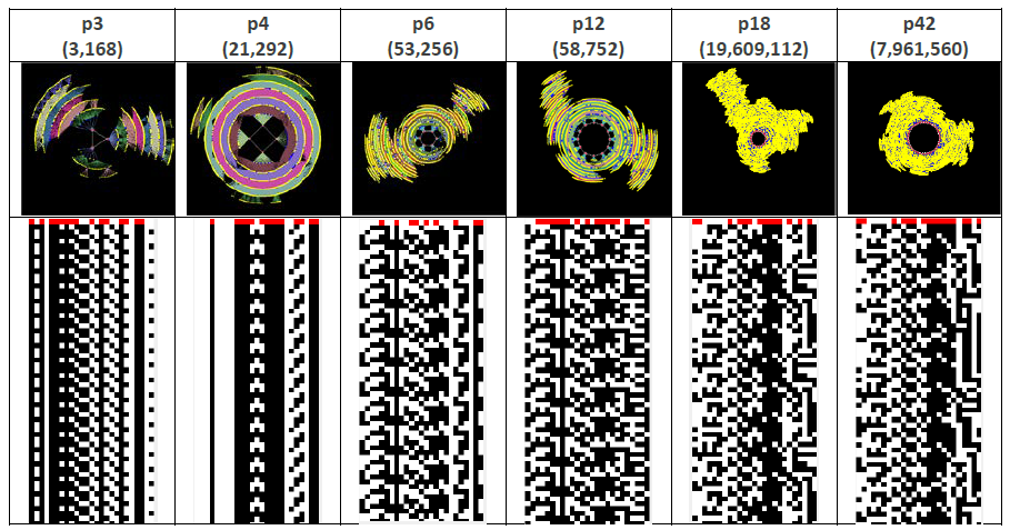
Figure 3 The phase space and state-time diagrams for 6 of the 20 attractors for the network of interest.
Node 0 is the right-most column, with Node 24 being the left-most.
Table 4 provides a summary of the phase space characteristics of this network. In short, there are 20 quantitatively different attractors, and 6 qualitatively different attractors (i.e., attractors with different periods) with periods ranging from 3 to 42. There is a single 18 period attractor that accounts for 58.4% of all phase space states, and the longest transient, i.e., the largest number of steps between a state not on an attractor basin (i.e., at the far end of an attractor transient branch), and a state on an attractor basin, is 117.
| Number of phase space attractors | 20 |
| Average period of phase space attractors | 8 |
| Longest period | 42 |
| Number of qualitatively different phase space attractors (different periods) | 20 |
| Number of qualitatively different phase space attractors (different structures) | 6 |
| Longest transient length | 117 |
| Largest number of pre-images | 208 |
| Average number of pre-images | 9.7027 |
| Garden-of-Eden percentage | 89.69 |
| Dynamical robustness | 0.594 |
| Size of largest attractor (relative to total size of phase space) | 0.5844 |
| Period of largest attractor | 18 |
Table 4 Summary of phase space characteristics of given network
An interesting metric in Table 4, which we won’t discuss much here, is Dynamic Robustness (DR). A DR of 0.594 says that, for nearly 60% of all network states, an external perturbation that flips the state of just one of the nodes will not result in a qualitative change in network behavior. Alternatively, for just under 40% of all network states, a small external force that flips the state of one node will push the network into a different attractor basin, i.e., the external force will result in a qualitative change in network behavior. DR is discussed in detail in Richardson (2009).
Dynamic Structure
You may have already noticed, from Figure 3, that some of the nodes seem to be fixed in the state-time diagram, i.e., their state does not change at all whilst in certain attractor basins. A fixed state suggests that no information is flowing through that node, or to put it another way, the multiple flows of information around the network conspire to ‘freeze’ some of the nodes. These nodes effectively become ‘walls of constancy’, or information barriers, through which no information flows.
An interesting characteristic of Boolean networks, and perhaps this extends to all complex networks, is that, as far as network function is concerned, any nodes that are frozen/inactive in all attractors can safely be removed without affecting the function - the qualitative structure of phase space - of the network (Richardson, 2005). For some networks (but not the one under study herein) the emergence of frozen nodes can result in the modularization of a network, in which the network is effectively carved-up into independent sub-networks. The point is that for any given attractor not all the nodes contribute, and so there is a sub-structure that is primarily responsible for the observed dynamics that is a subset of the overall network structure – static structure and effective dynamic structure can be very different indeed.
To illustrate this distinction further Figure 4 shows the effective dynamic structure for each of the attractors (functions) shown in Figure 3.
It is tempting to suggest that the nodes absent from each view contribute little to the network’s dynamical behavior. However, not only is it important to realize that a node that plays a small role in one function, may actually play a very special role in another (and all the possibilities in between), it is also essential to remember the importance of a ‘container’ for emergence to occur within.
In Glenda Eoyang’s Conditions for Self-Organizing in Human Systems (2001) thesis, she presents her CDE Model (Container/Difference/Exchange), in which the “Container bounds the system of focus and constrains the probability of contact among agents.” The inactive nodes in the network under study represent such a container within which the other nodes can interact and exchange information that contribute to the particular function that emerges. Notably, even though the whole network itself can be seen as a container (the very fact it is a network ‘contains’ the system considerably), the dynamic shape of that container is co-dependent on the attractor (function) being exhibited – the container itself is emergent; a node is ‘frozen’ as a result of the net effect of the 2345 interacting feedback loops.
Ensuring that removal of the frozen nodes left the compressed network functional equivalent to the original network would require checking that the node was frozen in every attractor. Even then, removal of the frozen nodes would still reduce the DR of the compressed network. So, compression needs to be considered in context. As we are analyzing the structural properties of the (dynamically) compressed graph in this paper, we do not have to apply such thorough criteria – fortunately, as checking all the attractors would be computationally intractable using the resources available to this stage of the research.
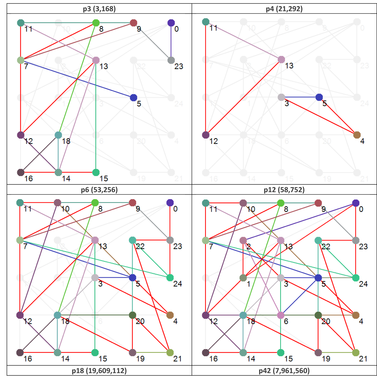
Figure 4 Effective dynamic structures for selected attractors. Note that the number in brackets after the attractor type is the number of states in phase space that map to that particular attractor. Red connections are bi-directional.
Power Graph Analysis (PGA)
Power graphs are novel representations of graphs, developed within the field of computational biology, that rely on two abstractions: power nodes and power edges. Power nodes are sets of nodes brought together and power edges connect two power nodes thus signifying that all nodes contained in the first power node are connected to all the nodes contained in the second power node. These language primitives allow for the succinct representation of stars, bicliques and cliques.
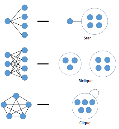
Figure 5 Power graph analysis primitives.
As Figure 5 shows, a star is expressed as a node connected via a power edge to a power node, a biclique is expressed as two power nodes connected by a power edge, and a clique is a power node connected to itself by a power edge. PGA does not concern itself with the direction of a connection – only that a connection exists.
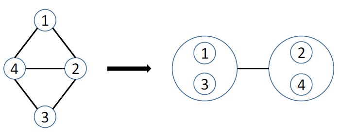
Figure 6 Simple power graph analysis example.
Figure 6 shows the result of applying power graph analysis (PGA) to a simple graph. The power graph representation reduces the number of edges needed to represent the network, groups together highly connected nodes as well as nodes having similar neighbors, and this without any loss of information. In the following, we will often use the notion of edge reduction, i.e., the proportion of edges that are abstracted from the original network in the power graph representation.
PGA is the computation and analysis of power graphs. Based on the work of Royer et al. (2008), an algorithm that computes power graphs is presented. Node clustering, module detection, network motif composition, network visualization, and network models can be recast in terms of PGA. PGA can be thought of as a lossless compression algorithm for graphs.
Compression levels of up to 95% have been obtained for complex biological networks. Microsoft and a team at Monash University have also looked at PGA (along with other edge compression techniques) as a way of simplifying complex software dependency graphs (Dwyer et al., 2013a, Dwyer et al., 2013b).
We will now examine the use of PGA to compress Boolean networks.
PGA of Boolean Networks
Figure 7 re-visualizes the diagrams in Figure 4 using PGA. The diagrams were generated using the CyOog plugin for Cytoscape (CyOog, 2012). Small grey numbered circles represent single nodes, black circles are power nodes and green power nodes are cliques.
Although PGA is most effective on vast networks containing 1000s of nodes we can see some simplifications when it is applied to these smaller graphs.
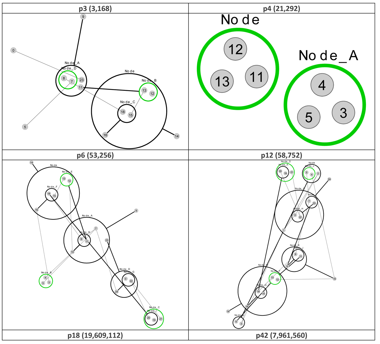
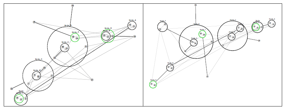
Figure 7 Power graph analyses of effective dynamic structures for selected attractors (see Figure 4).
The benefits of revisualization using PGA are more obvious with much larger networks, primarily because the degree of compression is considerably higher. With the relatively small network used for this study, the level of compression is minimal, but these alterative views do offer some structural insights that are not readily apparent from the traditional graph view. For example, although it would be difficult to say that the PGA view of the p3 (3,168) basin is any simpler than the equivalent traditional view offered in Figure 4, the fact that node groups 7, 8, 11, 23 and 12, 13, 15, 16, 18 represent two connected power nodes (in the language of PGA) may be of consequence.
We say ‘may’ because within the abstract framework we’re working within here understanding the significance of these power nodes is problematic. That being said, it would be interesting to see if targeting members of these power nodes leads to an increased probability of qualitative behavioral change within the network. This is a potentially interesting area for investigation in follow-up work.
We can also see, from a brief examination of p3 (3,168) and p6 (53,256) that nodes 9 and 14 are highly connected, and at the top of a hierarchy of power nodes. While the number of connections could have been obtained from a degree analysis, the relationships between the subgroups would have been lost. Nodes 8 and 9 both have degree 4, but it is clear that Node 9 is playing a different structural role than node 9 (? Something not right with this statement – need to fix). Also, the PGA makes it clear that Node 14 has links to a group of nodes with internal structure – the biclique of 16, 15 and 18.
It may be that nodes such as 9 and 14 act as levers to push the system into other attractors, but this would require further investigation. In addition, it is also notable that the set of nodes at the top of the power hierarchy varies between the different structural attractors (for p3 they are nodes 9 and 14; for p12 they are nodes 10, 14, and 24, etc.), suggesting that the nodes which are the most significant when considering interventions that might have the largest impact on dynamics, depends on which attractor basin the network is currently in – the best levers are determined by dynamic context. Looking at the dynamic robustness with particular focus on these nodes would also be of considerable interest.
In short, PGA has the potential to highlight areas of interest within a dynamic network that would benefit from deeper consideration.
Shannon Entropy as a Measure of Activity
Another way to partition (and so simplify) the network is to ‘layer’ it by considering the activity of each node. As a metric for activity we require a measure that was zero if the node state was ‘frozen’, and close to unity when the node was very active. After some trial and error, we found that the Shannon Entropy (https://en.wikipedia.org/wiki/Entropy_%28information_theory%29) of the state sequence for each node provided the appropriate activity profile – it provides a measure of the information contained in the node activity. The node state sequence is simply the state of a given node as it changes in time. So for a frozen node this might be ‘0,0,0,0,0,0,0,…’; this contains no information, and above is referred to as an information barrier.
The Shannon Entropy, H, of a particular node state sequence is calculated as:
Where P(x) is the proportion of 1s (or 0s) in the state sequence. Table 4 shows the Shannon Entropy for each node when the network is in each one of the attractor basins. The cells have been colored to indicate nodes with high Shannon entropy and those with low; the lowest being the red ‘frozen’ nodes. The table rows have been ordered by each node’s total entropy across all attractors, and the columns have been ordered by the number of red ‘frozen’ nodes in each attractor.
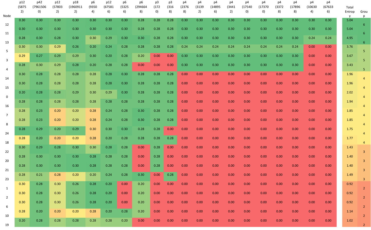

Table 4 Shannon Entropy for each node operating within each attractor basin.
Using the data presented in Table 4 allows us to ‘layer’ the network now in a different way, by grouping the nodes based on their Shannon Entropy, or activity. The group number is given in the last, rightmost, column. Similar to what is shown in Figure 4, Figure 8 provides six different views that, starting with group 6 (Nodes 11, 12 and 13 – the most active group), sequentially adds each group to the network structure until we arrive at the whole original network.
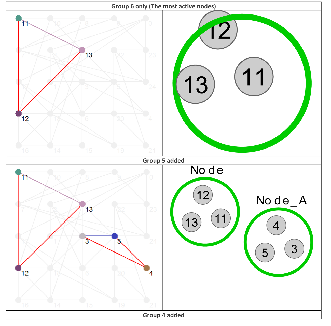
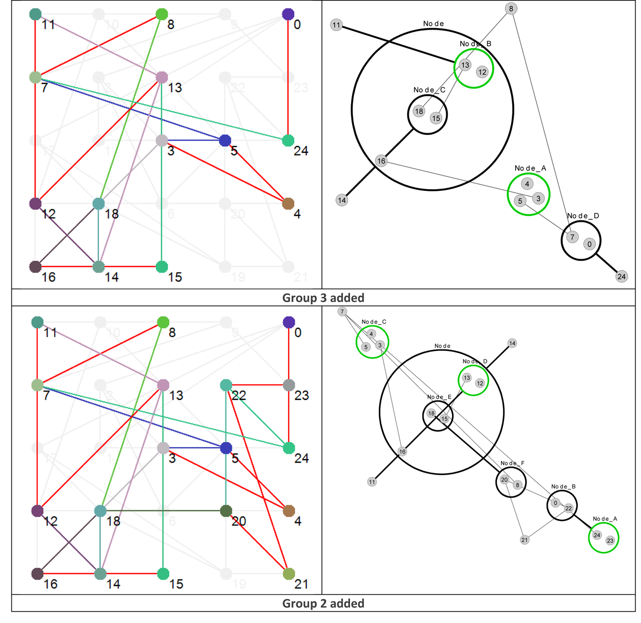
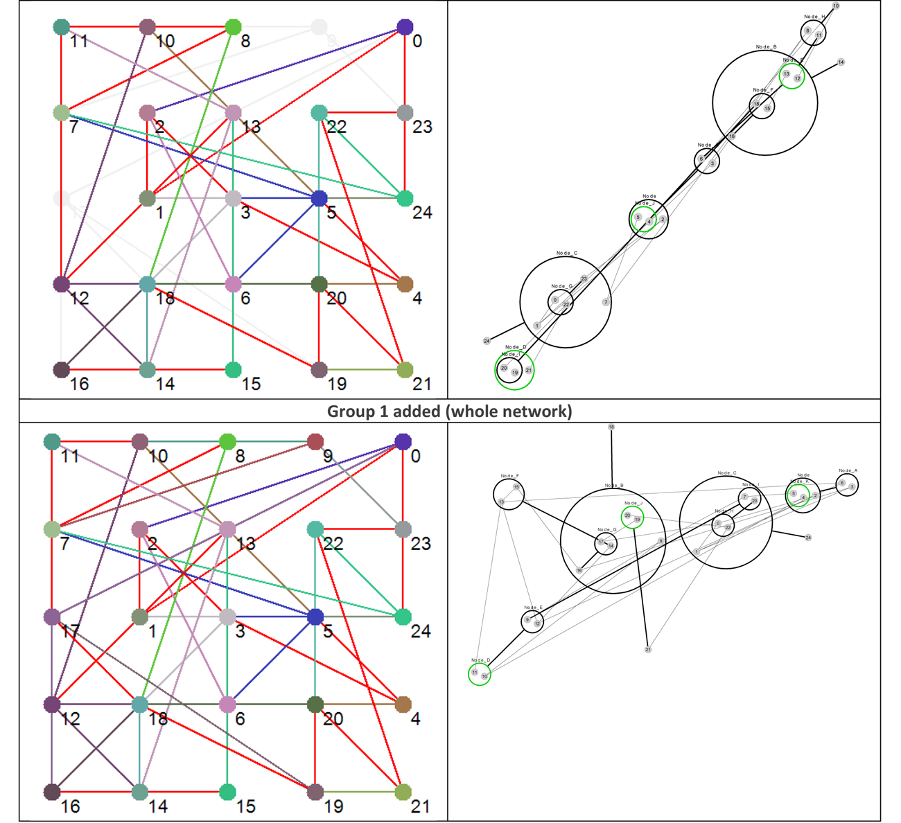
Figure 8 Effective dynamic layers based on node Shannon Entropy group.
Shannon Entropy Signatures (SESs)
Another way to visualize the dynamic behavior of the network of interest is to construct their Shannon Entropy (SE) profile or signature. For each attractor the SES is simply a column chart showing the SE for each node. Table 5 shows the SESs for four of the network’s attractors.
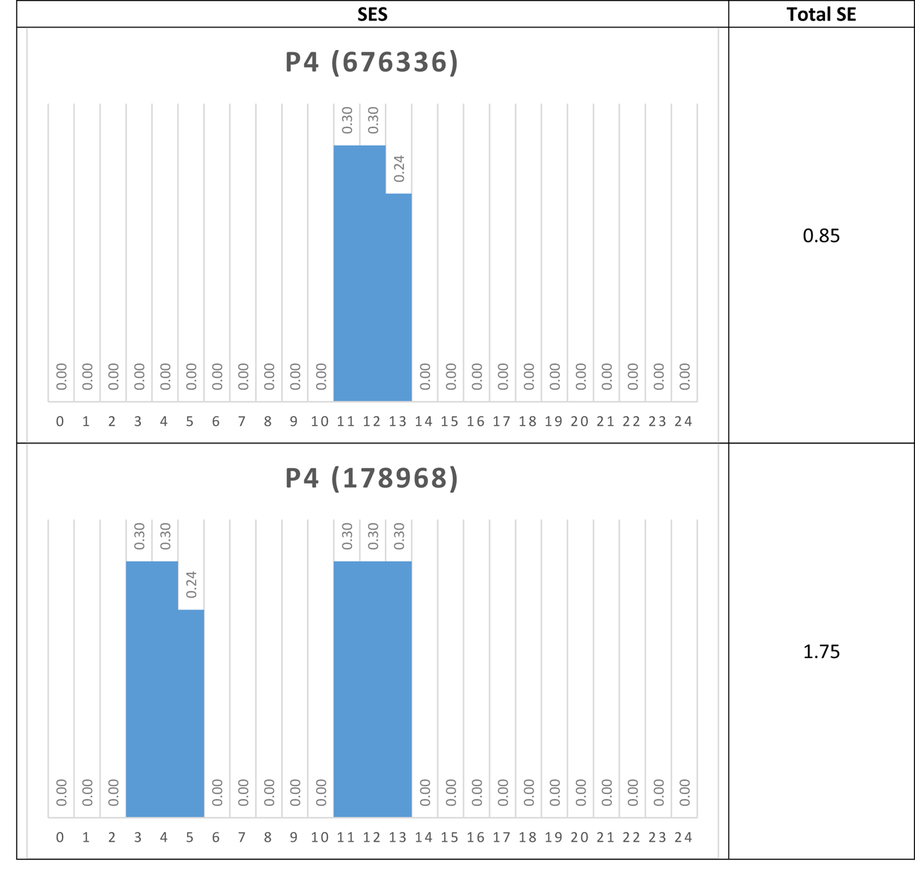
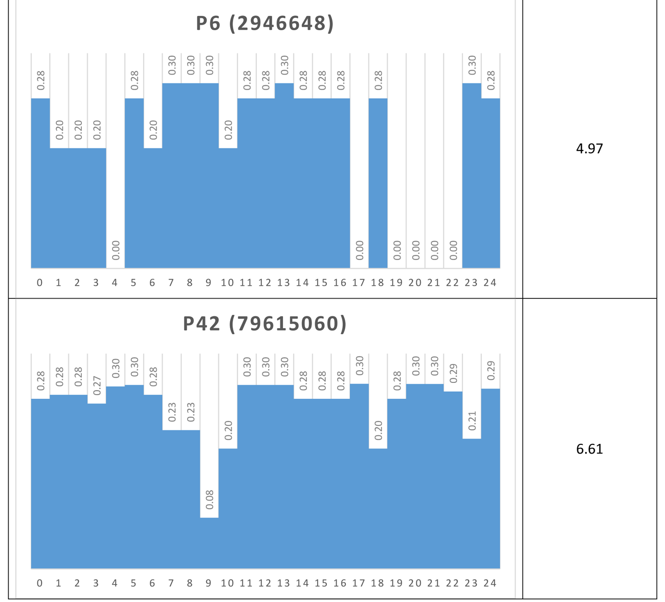
Table 5 Shannon Entropy Signatures for four attractors
Again, the dominant nodes in the p4 attractors are readily apparent.
If, via a small external perturbation, the network was pushed from a p4 attractor to a p42 attractor for example, we could say that the network has moved from a modular, low information (0.85) mode to a distributed, high information (6.61) mode. In this way, it may be possible to determine different operational modes in real networks, once a proxy for SE is determined.
Furthermore, rather than developing a set of archetypes for the different ‘connectivity modes’ and ‘information levels’ that the current network behavior might be mapped to, the focus would be on how the SES changes over time. In this way, we can monitor for qualitative changes in the SES, wave a flag to announce such a change, and then consider the significance within the network of interest of such an event.
Discussion and Conclusions
The aim of this paper in some ways is to make the obvious point that a pre-occupation with network structure in the absence of dynamic considerations (as is typical of traditional SNA) can lead to very misleading insights into how one might interact with a real-world complex network. In the presentation above it is clear that a purely topological analysis of the original network ‘graph’ would not capture some of the structural properties that only become apparent when dynamical, functional, and phase space analysis is performed.
Boolean networks were compressed by identifying their frozen nodes. We then looked at the use of power graph analysis (PGA) to further compress these networks. While PGA seems to achieve some simplification of network structure, the Boolean networks studied here were too small to clearly illustrate the full capabilities of PGA for network simplification. That being said, although the PGA views appear as complicated, if not more so in some cases, than the more traditional graph views, they do highlight different structural elements, such as stars and cliques more readily as well as hierarchically significant nodes.
Finally, a Shannon Entropy measure was applied to the networks, allowing them to be layered (from dynamical considerations) to aid visualization, while also providing a way of obtaining an information- based network signature. Further work will be required to see how these approaches can be applied to real-world dynamic networks.
Future work
The authors plan to develop this research in a number of areas. First, they intend port elements of the Boolean dynamic network analysis toolkit to a cloud-based web service. This will allow the study of larger networks, but also make the toolkit available to all academic researchers.
Once we have results for larger networks, PGA will be revisited to see if it is more effective in simplifying larger networks, and also to understand the identification of power nodes and the role they may play in network dynamics and robustness. We are also planning to further study the Shannon Entropy signature of various networks in an attempt to identify both valid proxies for the node state used herein, significant changes in network behavior. The authors believe that analysis tools based on this concept could be invaluable in areas such as security analysis and news reporting.
Finally, we hope to be able to start testing some of these approaches on real-world networks.
As mentioned in the introduction, some of the ideas herein are somewhat speculative, but we believe that by using insights from Boolean network analysis, robust general-use dynamic network tools can be developed.
Footnote
References
Borgatti, S.P., Everett, M.G., Johnson, J.C. (2013). Analyzing Social Networks, Sage Publications Ltd, ISBN: 978-1446247419.
Cilliers, P. (1998). Complexity and Postmodernism: Understanding Complex Systems, Routledge: London, UK.
CyOog (2012). http://www.biotec.tu-dresden.de/research/schroeder/powergraphs/download-cytoscape-plugin.html
Dwyer, T., Riche, N.H., Marriot, K., and Mears, C. (2013a). Edge Compression Techniques for Visualization of Dense Directed Graphs, Microsoft Research, http://research.microsoft.com/en-us/um/people/nath/docs/edgecompression_infovis2013.pdf
Dwyer, T., Mears, C., Morgan, K., Niven, T., Marriot, K., Wallace, M. (2013b), Improved Optimal and Approximate Power Graph Compression for Clearer Visualisation of Dense Graphs, arXiv:1311.6996 [cs.CG].
Economist (2015). The nuke detectives, Economist, 05 September 2015.
Eoyang, G. (2001). Conditions for Self-Organizing in Human Systems, http://www.hsdinstitute.org/about-hsd/dr-glenda/glendaeoyang-dissertation.pdf.
Kauffman, S. (1993). The Origins of Order: Self Organization and Selection in Evolution, Oxford University Press.
Magsino, S.L. Applications of Social Network Analysis for Building Community Disaster Resilience: Workshop Summary, The National Science Academies Press, ISBN: 978-0-309-14094-2.
Richardson, K.A. (2005). Simplifying Boolean networks, Advances in Complex Systems, ISSN 0219-5259, 8(4): 365-381.
Richardson, K.A. (2009). Robustness in complex information systems: The role of information 'barriers' in Boolean networks, Complexity, 15(3): 26-42.
Royer, L., Reimann, M., Andreopoulos, B., and Schroeder, M. (2008). Unraveling protein networks with power graph analysis, PLoS Comput Biol, 4(7): e1000108.