Complexity, Information and Robustness: The Role of Information ‘Barriers’ in Boolean Networks
Kurt A. Richardson
Abstract: In this supposed ‘information age’ a high premium is put on the widespread availability of information. Access to as much information as possible is often cited as key to the making of effective decisions. Whilst it would be foolish to deny the central role that information and its flow has in effective decision making, this paper explores the equally important role of ‘barriers’ to information flows in the robustness of complex systems. The analysis demonstrates that (for simple Boolean networks at least) a complex system’s ability to filter out, i.e., block, certain information flows is essential if it is not to be beholden to every external signal. The reduction of information is as important as the availability of information.
Introduction
In the Information Age the importance of having unfettered access to information is regarded as essential - almost a ‘right’ - in an open society. It is perhaps obvious that acting with the benefit of (appropriate) information to hand results in ‘better’ actions (i.e., actions that are more likely to achieve desired ends), than acting without information, although incidents of ‘information overload’ and ‘paralysis by (over) analysis’ are also common. From a complex systems perspective there are a variety of questions/issues concerning information, and its near cousin knowledge, that can be usefully explored. For instance, what is the relationship between information and knowledge? What is the relationship between information, derived knowledge, and objective reality? What information is necessary within a particular context in order to make the ‘best’ choice? How can we distinguish between relevant information and irrelevant information in a given context? Is information regarding the current/past state of a system sufficient to understand its future? Complexity thinking offers new mental apparatus and tools to consider these questions, often leading to understanding that deviates significantly from (but not necessarily mutually exclusive to) the prevailing wisdom of the mechanistic/reductionistic paradigms. In this paper, I would like to examine one particular aspect of information: How barriers to information, and its flow, are essential in the maintenance of a coherent functioning organization. My analysis will be necessarily limited. A very specific type of complex system will be employed to explore the problem, namely, Boolean networks. And, a rather narrow type of information will be utilized: a form that can be ‘recognized’ by such networks. Despite these and other limitations, I am confident that the resulting analysis has applicability to more realistic networks, such as human organizations, and that useful lessons can be gleaned from such an approach. At the end of the paper I shall briefly consider the shortcomings of the analysis offered and attempt to suggest how the conclusions might change when moving from abstract idealistic complex systems to concrete ‘messy’ human organizations. The paper begins with an introduction to Boolean networks and certain properties that are relevant to our analysis herein.
Boolean networks: Their structure and their dynamics
Given the vast number of papers already written on both the topology and dynamics of such Boolean networks there is no need to go into too much detail here. The interested reader is encouraged to look at Kauffman (1993) for his application of Boolean networks to the problem of modeling genetic regulatory networks. A short online tutorial is offered by Lucas (2006).
A Boolean network is described by a set of binary gates Si={0,1} interacting with each other via certain logical rules and evolving discretely in time. The binary gate represents the on/off state of the ‘atoms’ (or, ‘agents’) that the network is presumed to represent. So, in a genetic network the gate represents the state of a particular gene. The logical interaction between these gates would, in this case, represent the interaction between different genes. The state of a gate at the next instant of time (t+1) is determined by the k inputs or connectivity at time t and the transition function fi associated with site i:
There are 2k possible combinations of k inputs, each combination producing an output of 0 or 1.
Therefore, we have possible transition functions, or rules, for k inputs. For example, if we consider a simple network in which each node contains 2 inputs, there are 22=4 possible combinations of input - 00, 01, 10, 11 - and each node can respond to this combination of inputs in one of different ways. Figure 1 illustrates a simple example, showing the 4 different input configurations for each node and the 16 possible transition functions.
The state, or configuration, space for such a network contains 2N unique states, where N is the size of the network (so for the simple example shown, state space contains 64 states). Because state space is finite, as the system is stepped forward it will eventually revisit a state it has already visited. Combine this with the fact that from any state the next state is unique (although multiple states may lead to the same state, only one state follows from any state), then any Boolean network will eventually follow a cycle in state space. As a result, state space (or phase space) is connected in a non-trivial way, often containing multiple cyclic attractors each surrounded by fibrous branches of states, known as transients. Figure 2 shows the state space attractors, and their associated basins, for a particular Boolean network containing 10 nodes, each with 2 different inputs. The transition functions for each nodes were chosen randomly, but did not include the constant rules 0 (0000), or 15 (1111) as these force the node to be input-independent - nodes with constant transition functions do not change from their initial state.
Figure 2a shows the three attractors for this particular example: two period-1 attractor basins containing 32 and 672 states, respectively, and a single period-2 attractor basin containing the remaining 320 states (a total of 210=1024 states). In this example only four states actually lie on attractors and the remaining 1020 lie on the transient branches that lead to these four cycle states. Figure 2b is another way of visualizing how state space is connected. Each shade of grey represents one of the three attractor basins that together characterize state space. The figure comprises a grid with state 0000000000 at the uppermost left position and state 1111111111 at the lowermost right position. It shows, for example, that the 32 states that converge on the smallest period-1 (or, point) attractor are distributed in eight clusters, each containing four states. This particular representation is called a destination map, or phase space portrait, and we can see that even for small Boolean networks, the connectivity of state space is non-trivial. Figure 3 is a destination map for an N=20, k=3 Boolean network, to illustrate how quickly the complexity of state space connectivity increases as network size, N, increases. The boundaries between different shades are known as separatrices, and crossing a separatrix is a move from one attractor basin into another (adjacent) attractor basin.
It is all well and good to have techniques to visualize the dynamics that results from the Boolean network structure (and rules). But how is a network’s structure and its dynamics related? It is in the consideration of this question that we can begin to explore the role of information flows in such systems.
The potentially complex dynamics that arises from the apparently simple underlying structure is the result of a number of interacting structural feedback loops. In the Boolean network modeled to create the images in Figure 2, there are ten interacting structural feedback loops: two period-1, four period-2, one period-3, two period-4, and one period-5, or 2P1, 4P2, 1P3, 2P4, 1P5 for short. It is the flow of information around these structural loops, and the interactions between these loops that results in the three state space attractors in Figure 2; 2p1, 1p2 for short (here I use ‘P’ for structural loops and ‘p’ for phase space loops, or cycles). The number of structural P-loops increases exponentially (on average) as N increases, for example, whereas the number of state space p-loops increases (on average) in proportion to N (not as Kauffman, 1993, reported, which was found to be the result of sampling bias, Bilke & Sjunnesson, 2002).
For networks containing only a few feedback loops it is possible to develop an algebra that can relate P-space to p-space. However, as the number of p-loops increases this particular problem becomes intractable very quickly indeed, and the development of a linking algebra utterly impractical.
Sometimes the interaction of a network’s P-loops will result in p-space collapsing to a single period-1 attractor in which every point in state space eventually reaches the same state. Sometimes, a single p-loop will result whose period is much larger than the size of the network - such attractors are called quasi-chaotic (which can be used as very effective random number generators). Most often multiple attractors of varying periods result which are spread across state space in complex ways.
Before moving on to consider the robustness of Boolean networks, which will then allow us to consider the role information barriers play in network dynamics, it should be noted that state space, or phase space, can also be considered to be functional space. The different attractors that emerge from a network’s dynamics represent the network’s different functions. For example, in Kauffman’s analogy with genetic regulatory networks, the network structure represents the genotype, whereas the different phase space attractors represent the resulting phenotype, each attractor representing a different cell type. We can also regard the different attractors as different modes of operation, and an appreciation of a system’s phase space structure tells us about the different responses a system will have to a variety of external perturbations, i.e., it tells us which contextual archetypes the system ‘sees’ and is able to respond to.
Defining dynamical robustness
The dynamical robustness of networks is concerned with how stable a particular network configuration is under the influence of small external perturbations. In Boolean networks we can assess this measure by disturbing an initial configuration (by flipping a single bit/input, i.e., reversing the state of one of the system’s nodes) and observing which attractor basin the network then falls into. If it is the same attractor that follows from the unperturbed (system) state then the state is stable when perturbed in this way. An average for a particular state (or, system configuration) is obtained by perturbing each bit in the system state and dividing the number of times the same attractor is followed by the network size.
For a totally unstable state the robustness score would be 0, and for a totally stable state the robustness score would be 1. The dynamical robustness of the entire network is simply the average robustness of every system state in phase space. This measure provides additional information concerning how state space is connected in addition to knowing the number of cyclic attractors, their periods, and their weights (i.e., the volume of phase space they occupy).
For example, the average dynamical robustness of the network used to generate the data shown in Figure 2 is 0.825 which means the network is insensitive to 82.5% of all possible 1-bit perturbations. For the system used to generate the image in Figure 3, the dynamical robustness is 0.808.
More on structure and dynamics: Walls of constancy, dynamics cores and modularization
As we have come to expect in complex systems research, there is always more to the story than what first meets the eye. This is also the case which the issue of the relationship between network structure and dynamics. Although information flows (and is transformed) around the various structural networks, certain logical couplings ‘emerge’ that force particular nodes into one state or another, keeping them in that state for as long as the network is simulated. In other words, once the network is initiated and run forward, after some seemingly arbitrary period some nodes cease to allow information to pass. These ‘fixed’, or ‘frozen’ nodes effectively disengage all structural feedback loops that include them - although these structural loops still exist, they are no longer able to carry information around them. As such we can refer to them as non-conserving information loops. A number of such nodes can form ‘walls of constancy’ through which no information can pass, and effectively divide the network up into non-interacting sub-networks, i.e., the network is modularized. This process is illustrated in Figure 4.
The identification of these nodes is non-trivial (and even ‘non-possible’) before the networks are simulated. Although the effect is the same as associating a constant transition function with a particular node, the effect ‘emerges’ from the dynamic interaction of the structural feedback loops. It is a rare case indeed that these interactions can be untangled and the emerging frozen nodes identified analytically beforehand.
These ‘frozen’ nodes do not contribute to the qualitative structure of phase space, or network function. A Boolean network characterized by a 2p1, 1p2 phase space, like the one considered above, will still be characterized by a 2p1, 1p2 phase space after the frozen nodes are removed. In this sense, they don’t appear to contribute the networks function - they block the flow of information, but from this perspective have no functional role. Another way of saying this is that, if we are only concerned with maintaining the qualitative structure of phase space, i.e., the gross functional characteristics of a particular network, then we need only concern ourselves with information conserving loops; those structural feedback loops that allow information to flow around the network. This feature is illustrated in Figure 5 where the phase space properties of a particular Boolean network, and the same network after the non-conserving information loops have been removed (i.e., the networks ‘reduced’ form), are compared. Although the transient structure (and basin weight) is clearly quite different for the two networks, they both have the same qualitative phase space structure: 2p4.
The process employed to identify and remove the non-conserving loops is detailed in Richardson (2005a). As network size increases it becomes increasingly difficult to determine a network’s phase space structure. As such reduction techniques are not only essential in facilitating an accurate determination, but also in research that attempts to develop a thorough understanding of the relationship between network structure and network dynamics (as, already mentioned, only information conserving structural loops contribute to the network’s gross functional characteristics). Another term: what remains after all non-conserving loops (which includes associated ‘frozen’ nodes, and nodes that have no outgoing connections, or ‘leaf’ nodes) are removed from a particular network is known as the network’s dynamic core. A dynamic core contains only information conserving loops. So the majority of (random) Boolean networks comprise a dynamic core (which may be modularized) plus additional nodes and connections that do not contribute to the asymptotic dynamics of the network.
The role of non-conserving (structural) information loops
As the gross phase space characteristics of a Boolean network and its ‘reduced’ form are the same, i.e., (in this sense) they are functionally equivalent, it is tempting to conclude that non-conserving information loops - information barriers - are irrelevant. If this were the case then it might be used to support the widespread removal of such ‘dead wood’ from complex information systems, e.g., human organizations. The history of science is littered with examples of theories which once regarded such and such a phenomena as irrelevant, or ‘waste’, only to discover later on that it plays a very important role indeed. The growing realization that ‘junk DNA’ is not actually junk is one such example. What is often found is that a change of perspective leads to a changed assessment. Such a shift leads to a different characterization of non-conserving information loops. Our limited concern, thus far herein, with maintaining a qualitatively equivalent phase space structure in the belief that a functionally equivalent network is created, supports the assessment of non-conserving information loops as ‘junk’.
However, this assessment is wrong from a different perspective.
There are at least two roles that non-conserving information loops play in random Boolean networks:
- The process of modularization, and;
- The maximization of robustness.
Modularization in Boolean networks
We have already briefly discussed the process of modularization above. This process, which we might label as an example of horizontal emergence (Sulis, 2005), was first reported by Bastolla and Parisi (1998). It was argued that the spontaneous emergence of dynamically disconnected modules is key to understanding the complex (as opposed to ordered and quasi-chaotic) behavior of complex networks. So, the role of non-conserving information loops is to limit the network’s dynamics so that it does not become overly complex, and eventually quasi-chaotic (which is essentially random in this scenario: when you have a network with a high-period attractor of say 1020 - which is not hard to obtain - it scores very well indeed against all tests for randomness. One such example is the lagged Fibonacci random number generator).
In Boolean networks the resulting modules are independent of each other, so the result of modularization, is a collection of completely separate subsystems. This independency is different from what we see in nature, but the attempt to understand natural complex systems as integrations of partially independent and interacting modules is arguably a dominant theme in the life science, cognitive science, and computer science (see, for example, Callebaut & Rasskin-Gutman, 2005). It is likely that some form of non-conserving, or perhaps ‘limiting’, information loop structure plays an important role in real world modularization processes. Another way of expressing this is: organization is the result of limiting information flow.
Dynamic robustness of complex networks
Dynamic robustness was defined above, in a different way, as the stability of a network’s qualitative behavior in the face of external perturbations. In this section we will consider the dynamic robustness of an ensemble of random Boolean networks and their associated ‘reduced’ form to assess any difference between the two.
To do this comparison the following experiment was performed. 110,000 random Boolean networks with N=15 and k=2 (with random connections and random transition functions, excluding the two constant functions) were constructed. For each network its reduced form was determined using the method detailed in Richardson (2005a). The average dynamical robustness was calculated for both the unreduced networks and their associated reduced networks. The data from this experiment is presented in Figure 6, which shows the relationship between the average unreduced and reduced dynamic robustness for the 110,000 networks considered. (Error bars have not been added for reasons that are detailed later.) It is clear that on average the robustness of the reduced networks is noticeably lower than the unreduced networks. On average, the dynamic robustness of the reduced networks is typically of the order of 20% less than their parent (unreduced) networks. Of course, the difference for particular networks is dependent on specific contextual factors such as the number of non-conserving information loops in the (unreduced) networks (the extent of the dynamic core, in other words). This strongly suggests that the reduced networks are rather more sensitive to external perturbations than the unreduced networks. In some instances the robustness of the reduced network is actually zero meaning that any external perturbation whatsoever will result in qualitative change. What is also interesting, however, is that sometimes the reduced network is actually more robust than the unreduced network. This is a little surprising, but not when we take into account the complex connectivity of phase space for these networks. This effect is observed in cases when there is significant change in the relative attractor basin weights as a result of the reduction process and/or a relative increase in the orderliness of phase space. An example of this is shown in Figure 7.
The reason error bars are not added to the data is because in complex systems research it is important to consider the process of averaging data (and adding error bars extending a certain number of standard deviations). To illustrate this Figure 8a shows a more sophisticated representation of the raw ‘robustness’ data with the average superimposed (in black). The different colors indicate the number of data points that fall into a particular data bin (the data is rounded down to 3 significant figures). So red regions contain many data points (> a10 where a is the relative temperature of the data, a = 1.8 in this case) and dark blue regions contain only one (or a0) data point. It is clear that the data is multi-modal and as such we must be wary of using averages. Whereas Figure 8a includes all the data collected regarding unreduced and reduced dynamic robustness, Figures 8b – 8o show only the data for particular sizes of dynamic core. This helps considerably in understanding the detailed structure of Figure 8a. The various diagonal ‘modal peeks’ relate to networks with different dynamic core sizes, and the different horizontal structures correlate with networks containing smaller dynamic cores which can only display a fewer number of dynamic robustness values, i.e., as the size of the dynamic core decreases the data appears more discrete and as the core size increases the data appears more continuous (although there is still an upper bound to its resolution).
Further analysis was performed to confirm the relationship between network structure, dynamic core structure and, phase space structure. This included comparing the number of structural feedback loops in the overall network to the number of (information conserving only) loops in network’s dynamic core. Figure 9 shows the data for all (N=15, k=2) networks studied with all dynamic core sizes. The data indicates that on average the dynamic core of a network has between 30% and 60% fewer structural feedback loops; all of them information conserving loops. In the next section we shall consider the implications of this in terms of phase space characteristics and dynamic robustness.
Phase space compression and robustness
In Boolean networks, each additional node doubles the size of phase space. So even if ‘frozen’ nodes contribute nothing to longer term (asymptotic) dynamics, i.e., the number and period of phase space attractor, they at least increase the size of phase space. For example, the phase space of an N=20 network is 1024 times larger than an N=10 network. Thus, node removal significantly reduces the size of phase space. As such, the chances that a small external perturbation will inadvertently target a sensitive area of phase space, i.e., an area close to a separatrix, and therefore pushing the network into a different attractor, are significantly increased: a kind of qualitative chaos. This explains why we see the robustness tending to decrease when non-conserving information loops are removed.
Prigogine said that self-organization requires a container (self-contained-organization). The non-conserving information loops function as the environmental equivalent of a container. So it seems that, although non-conserving information loops do not contribute to the long term behavior of a particular network, these same loops play a central role as far as network stability is concerned. Any management team tempted to remove 80% of their organization in the hope of still achieving 80% of their yearly profits (which is sometimes how the 80:20 principle in general systems theory is interpreted) would find that they had created an organization that had no protection whatsoever to even the smallest perturbation from its environment – it would literally be impossible to have a stable business.
It should be noted that the non-conserving information loops do not act as impenetrable barriers to external signals (information). These loops simply limit the penetration of the signals into the system. For example, in the case of the modularization process, the products of incoming signals may, depending on network connectivity, still be fed from a non-conserving information loop into information conserving loops for a particular network module. Once the signals have penetrated a particular module, they cannot cross-over into other modules (as the only inter-modular connections are via non-conserving loops).
It should also be noted that, even though a particular signal may not cause the system to jump into a different attractor basin, it will still push the system into a different state on the same basin. The affect of signals that end-up on non-conserving information loops is certainly not nothing. So, although I use the term information ‘barriers’, these barriers are semi-permeable.
Balancing response ‘strategies’ and system robustness
Figure 10 shows a data histogram for the number of phase space attractors versus (unreduced) dynamic robustness. The plot shows that the robustness decreases rapidly initially as the number of phase space attractors increases. Remembering that the number of phase space attractors can also be seen as the number of contextual archetypes that a system ‘sees’, we see that versatility (used here to refer to the number of qualitatively different contexts a system can respond to, or is sensitive to) comes at the cost of reduced dynamic robustness assuming the same resources are available. Considered in this way robustness and versatility are two sides of the same coin. We would like for our systems to be able to respond to a wide variety environmental contexts with minimal effort, but this also means that our systems might also be at the beck and call of any environmental change. A system with only one phase space attractor doesn’t ‘see’ its environment at all, as it has only one response in all contexts, whereas a system with many phase space attractors ‘sees’ too much.
This is only the case though for fixed resources, i.e., given the same resources a system with few phase space attractors will be more robust than a system with a greater number. This is because, on average, the system with more phase space attractors will have a larger dynamic core and so the buffering afforded by non-conserving loops will be less pronounced. It is a trivial undertaking to increase phase space by adding nodes that have inputs but no outputs, or ‘leaf’ nodes (which is equivalent to adding connected nodes that have a constant transition function) – we might refer to this as a first-order strategy. This certainly increases the size of phase space rapidly, and it is a trivial matter to calculate the effect such additions will have on the network’s dynamical robustness, i.e., the increased dynamical robustness will not be an emergent property of the network. Increasing the robustness of a network (without changing the number, period and weight of phase space attractor basins) by adding connected nodes with non-constant transition functions is a much harder proposition. This is because of the new structural feedback loops created, and the great difficulty in determining the emergent ‘logical couplings’ that result in ‘frozen’ nodes which turn structural information loops that were initially conserving into non-conserving. It is not clear at this point in the research whether there is any preference between these two strategies to increase dynamical robustness, although one is orders of magnitude easier to implement than the other.
One key difference between the straightforward first-order strategy and the more problematic emergent strategy is that the first-order enhanced network would not be quantitatively sensitive to perturbations on the extra (buffer) ‘leaf’ nodes, i.e., not only would such perturbations not lead to qualitative change (a cross of a separatrix, or a bifurcation), but the position on the attractor cycle that the system was on when the node was perturbed (i.e., cycle phase) would also not be affected – there would no effect on dynamics whatsoever. This is because the perturbation signal (incoming information) would not penetrate the system further than the ‘leaf’ node, as by definition it is not connected via any structural (non-conserving or conserving) feedback loops: they really are impenetrable barriers to information. If the emergent strategy was successfully employed, the incoming signals would penetrate and quite possibly (at most) change the cycle phase, i.e., quantitative (but, again, not qualitative) change would occur. Either one of these response traits may or may not be desirable depending on response requirements.
To complete the data analysis Figure 11 shows three data histograms that show: (a) how the (unreduced) dynamic robustness varies with the number of information conserving loops; (b) how the size of the dynamic core varies with (unreduced) dynamic robustness, and; (c) how the size of the dynamic core varies with the number of information conserving loops. Figure 11a shows that on average a network’s dynamical robustness initially tends to decrease rapidly with the number of information conserving loops, but then quickly approaches saturation and stabilizes. Figure 11b shows this relationship from the difference perspective of dynamic core size rather than the number of information conserving loops connecting the elements of the dynamic core. This shows the average dynamic robustness decreasing steeply (and approximately linearly) for core sizes 0 to 3. The dynamic robustness continues to drop for core sizes > 3, but transitions to a very much slower rate (a rate which does increase slightly with increasing core size). Finally, Figure 11c shows that the average number of information conserving loops grows at an increasing rate with dynamic core size. Together these data show a preference for smaller dynamic core sizes (and hence lower numbers of conserving information loops, and therefore a higher proportion of non-conserving information loops). However, smaller dynamic core sizes lead to fewer phase space attractors and hence lower versatility as defined above. This, again, highlights the trade-off between flexibility and stability.
Conclusions and analytical limitations
From the analysis presented herein it is clear that non-conserving information loops - information barriers - are not ‘expendable’: they protect a system from both quantitative and qualitative (quasi) chaos. Quantitative chaos is resisted by the emergent creation of modules – through the process of modularization - which directly reduces the chances of phase space being dominated by the very long period attractors associated with quasi-randomness in Boolean networks. Whereas qualitative chaos - the rapid ‘jumping’ from one attractor basin to another in response to small external perturbations - is resisted by the expansion of phase space, which reduces the possibility of external signals pushing a system across a phase space separatrix.
As mentioned at the beginning of this paper, there are certain limitations to the use of Boolean networks as surrogates for real world organizations. To close this paper, I’d like to briefly consider some obvious limitations, strategies and implications for overcoming them.
Perhaps the most obvious shortcoming is the simplicity of the transition functions themselves. However, although Boolean networks only allow each node to adopt two different states, there is nothing fundamentally different about extending the analysis to include an arbitrary number of different states, and an arbitrary degree of transition function complexity. The important step is the discretization of state space. As such we wouldn’t expect the results presented herein to change fundamentally.
A trickier shortcoming to address is the fact that in these discrete systems each node has only one identity, and so there is only one response to any particular signal. In human systems, there is plenty of evidence to suggest that human decision-makers adopt one of several different identities depending on certain contextual factors. There are (at least) to ways to address this shortcoming. The easy way is to assume that the modeled structure is valid only for periods shorter than the average time between ‘identity shifts’. This would be an interesting parameter to enumerate! Another, more sophisticated approach would be to represent each node as a sub-network itself for which the different sub-network attractors would represent different identities1. Again, as long as state space is discrete, we would still expect to see the emergence of non-conserving information loops and a similar role for them.
This strategy of increasing the complexity of transition functions and reframing what we consider a ‘node’ to be (either a single node or a connected sub-network) can potentially even be employed to make the (seemingly non-adaptive) network appear to be adaptive, with changing connectivity at some levels, new entities emerging, and evolving identities. The frame of reference from which the network is considered enables these features to be ‘seen’ or not. Again, the important element is discretization of state space. I explore this particular issue of the relationship between non-adaptivity and adaptivity in discrete systems at much greater detail in Richardson (2005b). What would become a challenge as we arbitrarily increased the complexity of such networks (other than the considerable challenge of actually constructing and running them) is not that the fundamental importance of non-conserving information loops would diminish, but that the physical interpretation of them would change as we ‘stood further back’ from the network. If we take this to the extreme, assume that a network model of fundamental matter is correct - an exquisitely complex network of simply connected simple entities (supernodes?) - then what role do non-conserving information loops (at that fundamental level) play at the human level? And what is the equivalent to non-conserving loops (at the fundamental level) at other levels of ‘reality’? I certainly won’t try to answer these questions here (partly because I believe they have so many different answers).
My reason for ending the paper on such a philosophical note is to simply warn against the temptation to dismiss the results of a particular analysis just because the model appears to be too simplistic. There is a deeply profound relationship between simplicity and complexity that scientists (and all variety of thinkers) are only just beginning to understand. That being said, it might be that very simple models are more suitably employed as metaphors rather than analogies. If we chose to use the Boolean network model as a direct analogy (which I certainly think is possible at a much higher level of compositional complexity) we might find that the exact idea of a ‘non-conserving information loop’, for example, is so abstract that it would make a useful physical interpretation incredibly difficult to extract. If however, we chose to regard the model as a useful2 metaphor then we are free to exploit the idea of a ‘non-conserving information loop’ (for example) without feeling obliged to stay honest to its exact (in the Boolean framework) definition; it becomes a useful tool for thinking rather than a tool to replace our useful thinking.
To conclude, I would suggest that ‘barriers’ (both impenetrable and semi-permeable) to information flow play an important role in the functioning of all complex information systems. However, the implications (and meaning) of this for real world systems is open to many different interpretations. At the very least it suggests that ‘barriers’ to information flow should be taken as seriously as ‘supports’ to information flow (although, paradoxically, a good ‘supporter’ is inherently a good ‘barrier’!)
Footnotes
References
Bastolla, U. and Parisi, G. (1998). “The Modular Structure of Kauffman Networks,” Physica D, ISSN 0167-2789, 115: 219-233.
Bilke, S. and Sjunnesson, F. (2002). “Stability of the Kauffman model,” Phys. Rev. E, ISSN 1063-651X, 65: 016129.
Callebaut, W. and Rasskin-Gutman, D. (2005). Modularity: Understanding the Development and Evolution of Natural Complex Systems, Cambridge, MA: MIT Press.
Kauffman, S. A. (1993). The Origins of Order: Self-Organization and Selection in Evolution, New York, NY: Oxford University Press, ISBN 0195058119.
Richardson, K. A. (2005a). “Simplifying Boolean networks,” Advances in Complex Systems, ISSN 0219-5259, 8(4): 365-381.
Richardson, K. A. (2005b). “The Hegemony of the Physical Sciences: An Exploration in Complexity Thinking,” Futures, 37: 615-653.
Sulis, W. H. (2005). “Archetypal Dynamical Systems and Semantic Frames in Vertical and Horizontal Emergence,” in K. A. Richardson, J. A. Goldstein, P. M. Allen and D. Snowden (eds.), E:CO Annual Volume 6, Mansfield, MA: ISCE Publishing, ISBN 0976681404, pp. 204-216.
Kurt A. Richardson is the Associate Director for the ISCE Group and is Director of ISCE Publishing, a new publishing house that specializes in complexity-related publications. He has a BSc(hons) in Physics (1992), MSc in Astronautics and Space Engineering (1993) and a PhD in Applied Physics (1996). Kurt’s current research interests include the philosophical implications of assuming that everything we observe is the result of complex underlying processes, the relationship between structure and function, analytical frameworks for intervention design, and robust methods of reducing complexity, which have resulted in the publication of over 25 journal papers and book chapters. He is the Managing/Production Editor for the international journal Emergence: Complexity & Organization and is on the review board for the journals Systemic Practice and Action Research, Systems Research and Behavioral Science, and Tamara: Journal of Critical Postmodern Organization Science. Kurt is the editor of the recently published Managing Organizational Complexity: Philosophy, Theory, Practice (Information Age Publishing, 2005) and is co-editor of the forthcoming books Complexity and Policy Analysis: Decision Making in an Interconnected World (due June 2006) and Complexity and Knowledge Management: Understanding the Role of Knowledge in the Management of Social Networks (due January 2007).
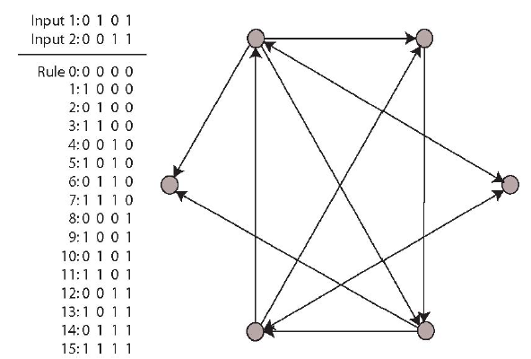
Figure 1 A simple Boolean network
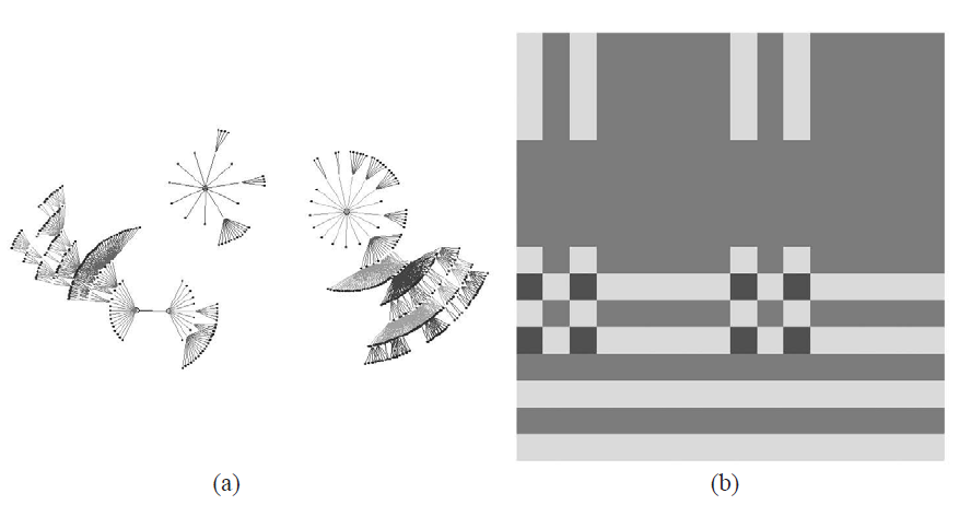
Figure 2 The state space of a small Boolean network
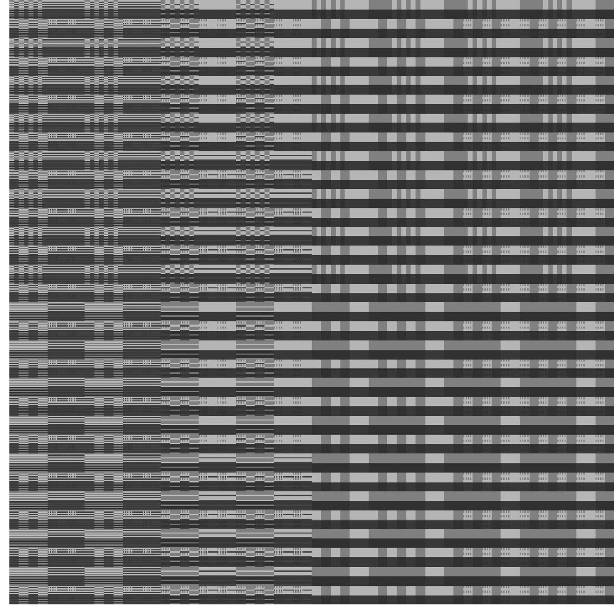
Figure 3 An example of a destination map for an N=20, k=2 Boolean network
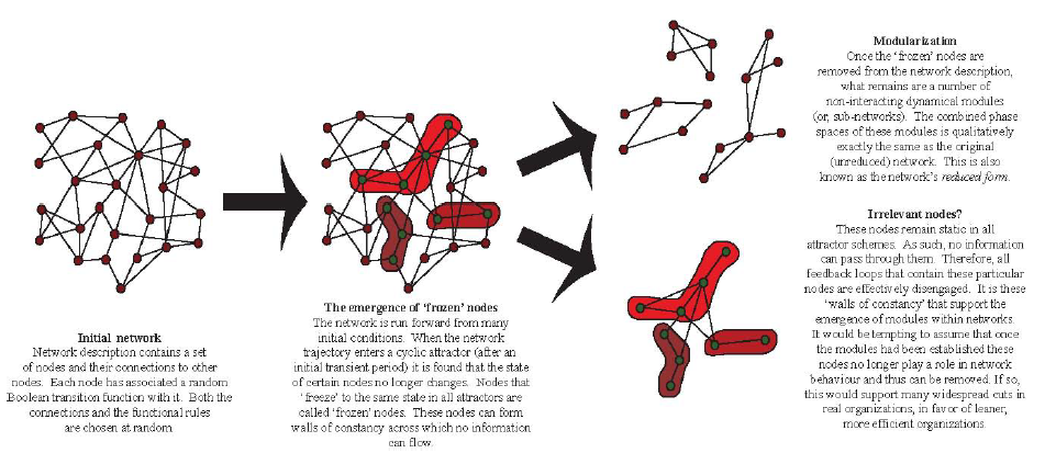
Figure 4 The process of modularization in complex networks
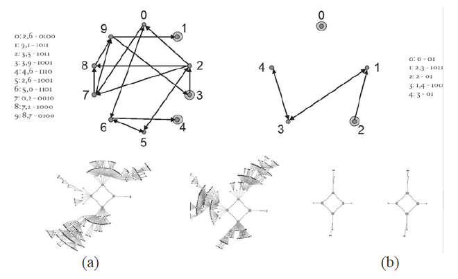
Figure 5 An example of (a) a Boolean network, and (b) its reduced form. The nodes which are made up of two discs feedback onto themselves. The connectivity and transition function lists at the side of each network representation are included for those readers familiar with Boolean networks. The graphics below each network representation show the attractor basins for each network. The phase space of both networks contain two period-4 attractors, although it is clear that the basin sizes (i.e., the number of states they each contain) are quite different.
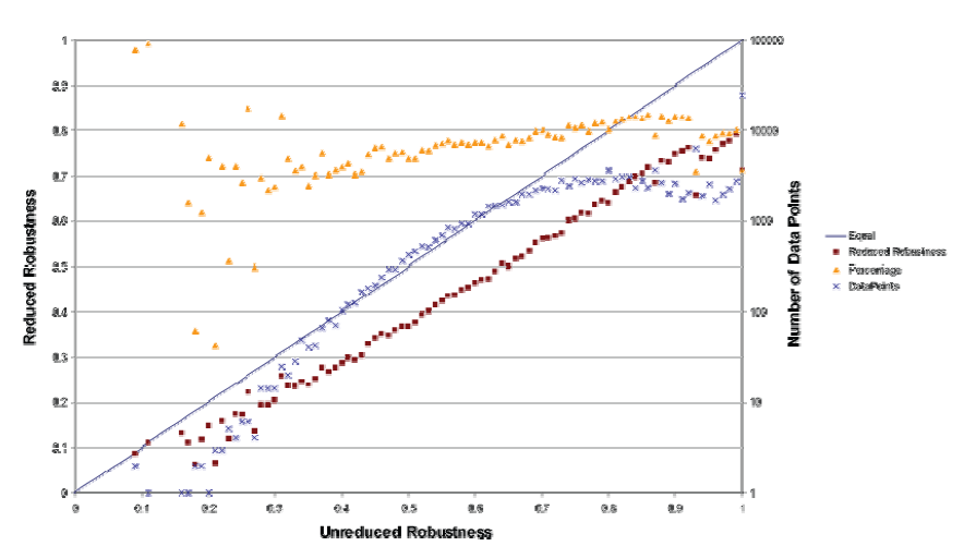
Figure 6 The average relationship between unreduced dynamic robustness and reduced dynamic robustness. The ‘DataPoints’ line shows the number of data points that comprise each calculation of the average. The ‘Percentage’ line shows the ratio (reduced robustness)/(unreduced robustness). The line unreduced robustness = reduced robustness is also indicated (‘Equal’).
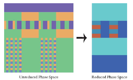
Figure 7 An example of when dynamical robustness actually increases when a complex network is reduced
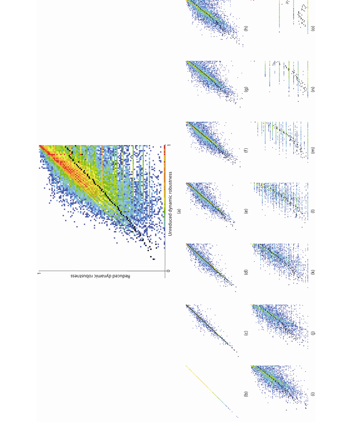
Figure 8 A detailed viewed of the dynamical robustness data collected. (a) all data, with black points showing the overall average, (b) data associated with a dynamic core size of 15, (c) 14, (d) 13, (e) 12, (f) 11, (g) 10, (h) 9, (i) 8, (j) 7, (k) 6, (l) 5, (m) 4, (n) 3, and (o) 2.
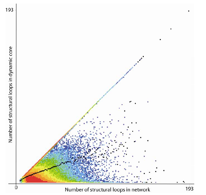
Figure 9 A ‘temperature plot’ showing the relationship between the number of structural feedback loops in the unreduced networks, and the number of active structural loops in their dynamic cores. The black points represent the average number of structural loops in dynamic core.
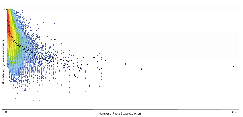
Figure 10 A data histogram showing the relationship between the number of phase space attractors and the (unreduced) dynamical robustness. The black points represent the average dynamic robustness for increasing numbers of phase space attractors.
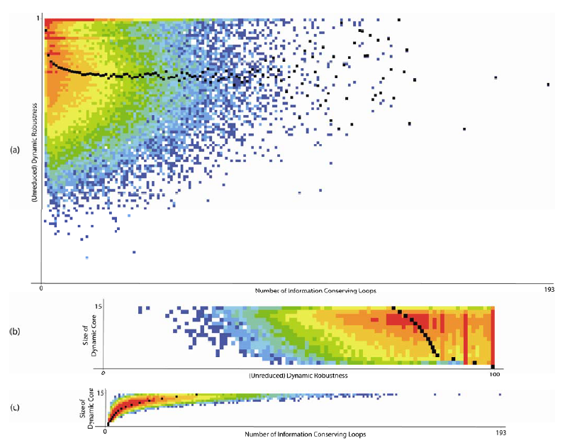
Figure 11 Data histograms showing the relationship between: (a) the number of information conserving loops and the (unreduced) dynamic robustness (black points represent the average dynamic robustness); (b) the (unreduced) dynamic robustness and the size of the dynamic core (black points represent the average dynamic robustness for given dynamic core size), and; (c) the number of information conserving loops and the size of the dynamic core (black points represent the average number of information conserving loops for given dynamic core size).