REFLEX INHIBITION BY DORSAL ROOT INTERACTION12 [127]
B. Howland, J.Y. Lettvin, W.S. McCulloch, W. Pitts and P.D. Wall
Introduction
Ballif et al. (1), in 1925, found that a single shock to a mixed ipsilateral hind-limb nerve of a spinal or decerebrate cat inhibited the knee-jerk for hundreds of milliseconds, and they said that the cause of this phenomenon was still to be elucidated. In 1938, Barron and Matthews (2) found that stimulation of an ipsilateral dorsal root often inhibited ventral root response to stimulation of a second dorsal root, and they were the first to suggest that blocking at the bifurcation of primary afferent neurons might account to some extent for their finding. Renshaw (3), in 1946, using volleys over dorsal roots L6 and L7, showed that the inhibition was accompanied by changes in that part of the microelectrode record from the ventral horn which he attributed to the presynaptic components. The early course of the inhibition was not paralleled by any change in the responsiveness of motoneurons to antidronic stimulation; hence he attributed it to an interaction between terminal branches of dorsal root fibers.
In the same year, Eccles and Malcolm (4) observed in the frog that the dorsal root reflex and DR5 were inhibited and they suggested that the conditioning volley produced a cathodal block of the primary afferent fibers by a depolarization spreading back from the synaptic region. Granted that this is the cause of the phenomenon, the evidence for it is indirect and of such a kind that it cannot localize the block exactly. Therefore it seemed advisable to examine the events within the cord by a method that can show directly at what place the afferent volley is first diminished. Although the inhibition has been seen after peripheral nerve stimulation in both decerebrate and spinal animals without anesthesia, it is more prolonged and profound under barbiturates and with dorsal root stimulation. We used the latter preparation.
For physical reasons records from the roots and from the surface of the cord do not determine uniquely the site of electrical events within the cord. A grid of successive stations of microelectrodes was used to produce a series of potential maps, each of effectively simultaneous values, showing the fields of the inhibitory volley remaining at the time of maximum inhibition and those engendered by the test volley alone and inhibited. These maps indicate the potentials in the extracellular medium at enough points to permit calculation of the amount of current flowing into or out of the neurons in small regions. Thereby we estimate to what extent those small regions are the sites of impulses, absorbing current from the medium (i.e., sinks), or sites contributing current through the medium (i.e., sources) to impulses in their remote parts. Computations and the justification of their use in determining location of activity in the central nervous system, being novel, are discussed at some length.
To present the significant results of each experiment requires many figures, so we shall present the results of a single typical one in detail. All the experiments show during dorsal root inhibition that the test volley in the primary afferent neurons is much diminished before it reaches the grey matter of the spinal cord. They do not show by what agency—internuncials or other fibers directly—this inhibition is exerted on the primary afferent fibers.
Preparation
A cat was anesthetized with Dial-Urethane, 0.6 cc. per kg. intraperitoneally. A tracheal cannula was installed and artificial respiration established. The spinal cord was transected at C1. Heating lamps controlled by a subscapular thermistor maintained the body temperature at 38°C ±0.1°C. The lumbar enlargement was exposed and covered with mineral oil continuously suffused with 95 per cent O2 + 5 per cent CO2. Dorsal roots L5 and L6 on one side were severed about 3 cm. from the cord and placed on bipolar electrodes for test and conditioning stimulation respectively. Dorsal root potentials were recorded on a filament dissected from one of the stimulated roots, and the ventral root response was led from the severed ipsilateral VR of L6. Throughout the experiment supramaximal shocks of 0.1 msec. duration were delivered every 2 sec. through isolating transformers.
By varying the interval between the conditioning volley on L6 and the testing volley on L5, the ventral root response to the test volley was found to be inhibited at all intervals between 5 and 100 msec., and maximally at about 20 msec. This interval between conditioning and test stimulus was maintained thereafter throughout the experiment. Additional Dial was given then to decrease spontaneous and evoked activity within the cord. In due time the ventral root discharge vanished and never reappeared. During the recording, after the second dose of Dial, many internuncials were encountered which responded, frequently repetitively, to the test volley alone. Their response was much diminished by a prior conditioning volley. Apparently, despite the heavy anesthesia and silent ventral roots, impulses in the primary collaterals were capable of causing related activity in internuncials and the conditioning volley was still able to inhibit them. The monitoring dorsal root filament response changed a little, and then became and remained constant, thus indicating the stability of the preparation throughout the recording.
Experiment
Records of potentials throughout a transverse plane in the ipsilateral half of the spinal cord a few millimeters rostral to L5 were obtained through microelectrodes made of 10 µ platinum wire uniformly coated with a thin layer of glass and sharpened (5). The first electrode was placed on the intact pia of the dorsum of the cord under binocular microscopic vision to insure that there was no dimpling of the surface at the time of contact or at any subsequent time. The electrical response at the surface was then recorded on a quiet base line nine times: thrice of the conditioning volley alone, thrice of the test volley alone, and thrice of the combination of the test volley 20 msec. after the conditioning volley. The electrode was then advanced 150 µ into the cord and the full series of nine records taken again. This procedure was repeated in steps of 150 µ until the tip of the electrode reached its final station some 3 mm. deep in the cord. Still under binocular microscopic observation, its shank was carefully severed, its cut end checked for approximation, and its shaft left in place. Ten electrodes were thus introduced, of which nine are shown in Fig. 1. This took several hours, during which there was no visible change in the monitoring root records.
The microelectrode records were all taken with respect to a retractor separating the back muscles; the calculations subtract its contribution to all the measured potentials. The microelectrodes were connected to a cathode-follower with grid current less than 10-11 A., grid-ground leak of 1011 O., and the capacitative shunt from grid to ground balanced by a negative capacitance. Hence any difference of impedance between electrode tips had negligible effect. The output of this head-stage went to a capacity-coupled amplifier with a bandwidth of 0.5–100,000 cycles, and thence to an oscilloscope with a linear sweep. To avoid distortion by parallax, only the center 3 inches of the 5-inch screen were used. On each record a stimulus artefact had to be introduced for temporal reference and a base line for amplitude measurement had to be superimposed by an additional sweep with the input to the scope grounded. Each record is a single frame photographed on 35-mm. film.
When the experiment was finished the cord was fixed in situ with 10 per cent formalin, and 24 hrs. later a slab, 1 mm. thick and containing all the electrodes, was removed into 10 per cent formalin for another 24 hrs. It was next carefully dehydrated with alcohol in several steps for three days and then placed in several changes of 100 per cent alcohol for three more days. Finally, it was cleared in methyl salicylate, which made the slab so transparent that the outlines of the grey matter and the exact position of the electrodes in the transverse plane could be seen and photographed. The linear shrinkage was less than 5 per cent, and when the micrometer readings for depth of penetration were checked against the histological measurements, four electrodes agreed exactly, five with an error less than 5 per cent, and only one had deviated from the plane and had to be disregarded.
Results
Figure 1 shows the positions of the 162 recording stations used in computation. The observations were now embodied in nearly 1500 records, from which the significant results were extracted as follows: Since inspection of all responses to the conditioning volleys alone showed that the potentials changed little, if at all, from 20 to 23 msec. after the shock, a single map was prepared for this interval by plotting the mean of the three records at that time at each station on an enlarged replica of Fig. 1. Similar charts were made at each of the instants 1.0, 1.2, 1.6, and 2.8 msec. after the test shock alone and after the combination consisting of the test shock preceded 20 msec. earlier by the conditioning shock. Figure 1 was projected on squared paper at such enlargement that the distances between recording stations was about the same as the unit square of the paper, and this figure was blueprinted in many copies. Potential values at the intersections of the lines of the paper, or “lattice points,” were then determined by interpolation, accurate enough to preserve second differences, first along the electrode tracks to the horizontal lines of the squared paper, and then along the horizontal lines to the lattice points, where the values were entered numerically. From each of these square arrays of values two diagrams were made. The lower are isopotential maps at the indicated times, and contain the relevant information, but in a form from which it is difficult to determine, by inspection, where activity is, or how it is moving. The upper diagrams are made by entering, at each lattice point, the difference between the potential there and the average at the four neighboring lattice points. The value of this difference is indicated by the number of dots or diagonal lines in a group, the dots standing for negative, the lines for positive values. One dot or line is chosen to be approximately the standard error of the quantity, so that groups of less than three may be due to error. Where there are dots, their density is an approximate measure of activity indicating the extent to which parts of neurons there absorb current from the medium (i.e., sink density). The density of lines indicates the extent to which parts of neurons there emit current into and through the medium to other depolarized parts of the same neurons (i.e., source density). A source signifies that the region has been or is about to be a sink. The maps summarize the findings.
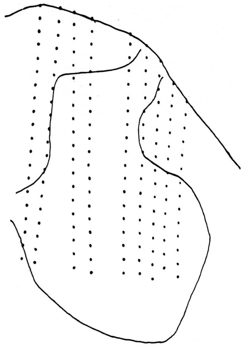
Figure 1. Tracing of cross section of cat spinal cord between L4 and L5 showing the 162 positions from which the potentials were recorded. Area analyzed is approximately 2.7 mm. by 1.8 mm.
Map C 20 msec. after conditioning stimulus to L6 alone (Fig. 2, C 20 msec.)
At this time, and with no change in magnitude for at least 3 msec. more, the bulk of residual activity is along the dorsal border of the dorsal horn— the sinks chiefly in the grey matter, the sources chiefly in the white.
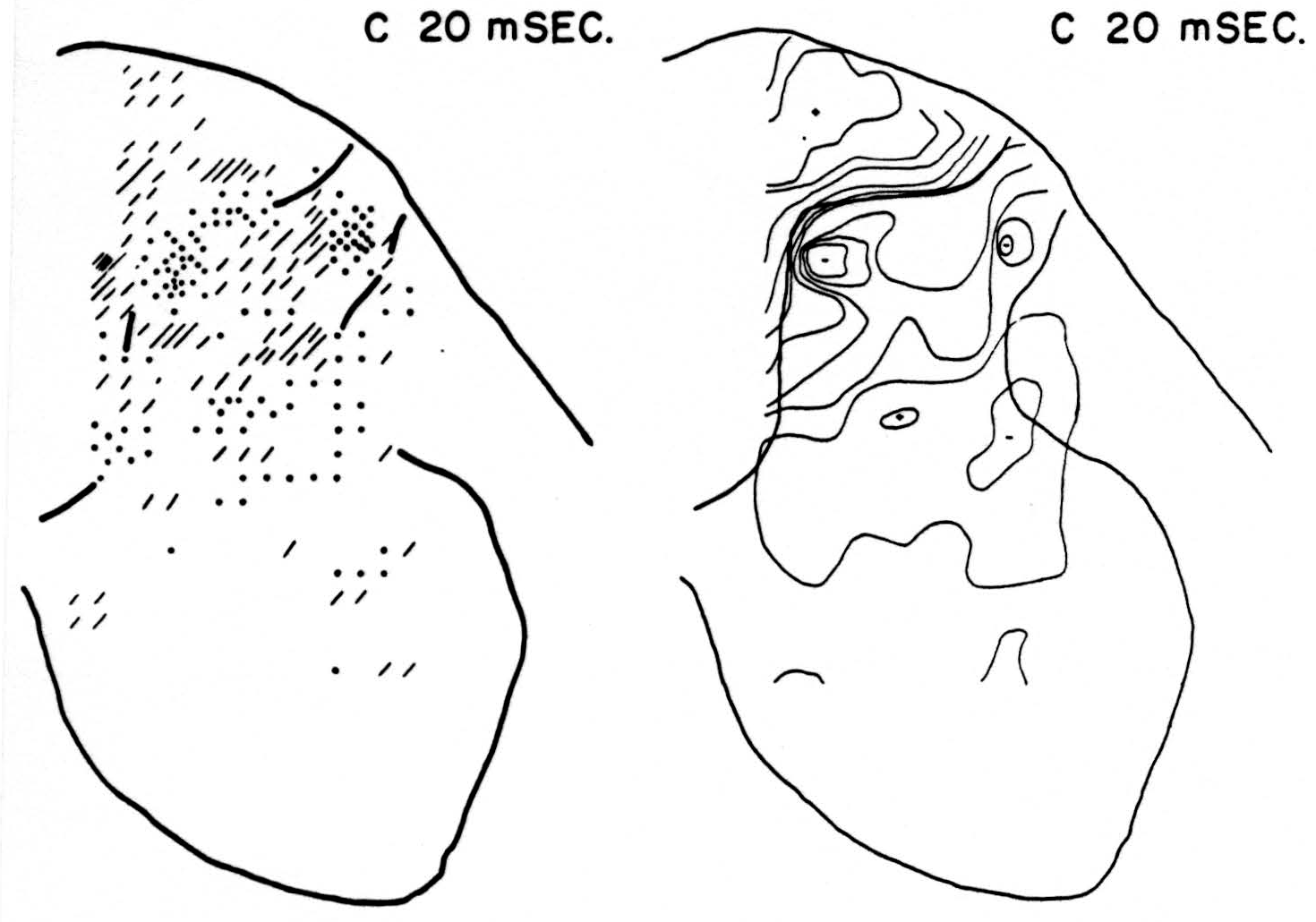
Figure 2. Right: distribution of isopotentials within spinal cord 20 msec. after conditioning root L6, alone, had been stimulated. This time was found to be that at which stimulation of root L6 exerted its maximum inhibitory effect on reflex following stimulation of test root L5. Left: distribution of sources (diagonal lines) and sinks (dots) within spinal cord 20 msec. after stimulation of conditioning root. Each dot or line represents an equal amount of source-density. For interpretation see text.
Maps T after test stimulus to L5 alone (Figs. 3-5, T 1.2, T 1.6, T 2.8 msec.)
No maps are presented for 0.5 or for 1.0 msec. after the test stimulus alone because, although there was a large potential gradient in the plane, there were as yet no significant sources or sinks, showing that the volley had not yet reached the plane. At 1.2 msec. (Fig. 3, T 1.2 msec.), the volley from the medial division of the dorsal root is represented by a line of sinks in the dorso-medial white matter just entering the grey. At this time the grey matter contains mainly sources, except for regions perhaps excited slightly earlier by faster afferents. At 1.6 msec. (Fig. 4, T 1.6 msec.), the medial sinks have invaded the adjacent grey matter in force, and a large sink has appeared in the dorso-lateral grey; and by 2.8 msec. (Fig. 5, T 2.8 msec.), intense sinks are present in the substantia gelatinosa and in the medial and lateral intermediate region.
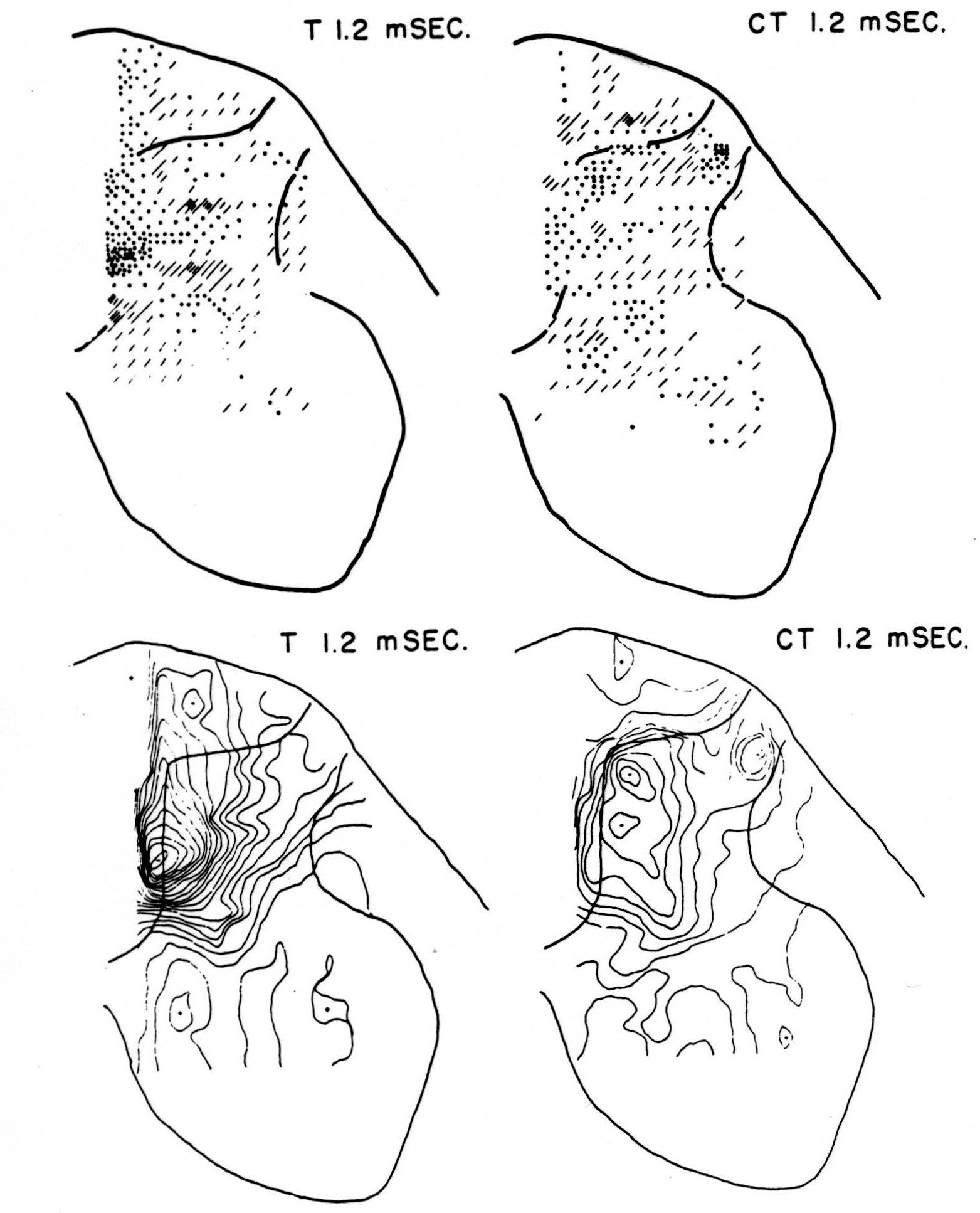
Figure 3. Top left: distribution of sources (lines) and sinks (dots) 1.2 msec. after test root L5, alone, had been stimulated. This is pattern of earliest disturbance recorded in region after test stimulation. Bottom left: isopotential map 1.2 msec. after stimulation of L5 alone. Top right: source-sink map 1.2 msec. after stimulating test root but preceded 20 msec. by stimulation of inhibitory conditioning root L6. This shows that earliest sign of arriving volley in white matter is inhibited by preceding volley. Bottom right: isopotential map 1.2 msec. after stimulating test root but preceded 20 msec. earlier by conditioning volley.
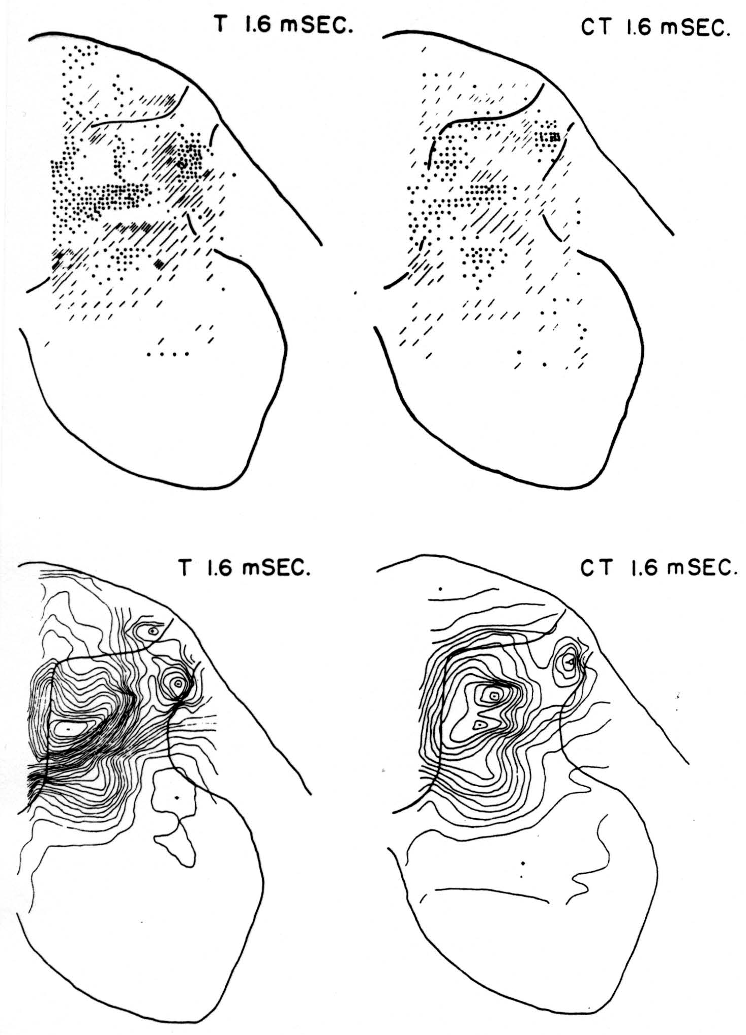
Figure 4. Arranged as in Fig. 3; top left, source-sink distribution, and bottom left, isopotential distribution, 1.6 msec. after stimulation of test root L5. Top right, source-sink map, and bottom right, isopotential map, at the same time after test volley but preceded 20 msec. by inhibitory conditioning volley.
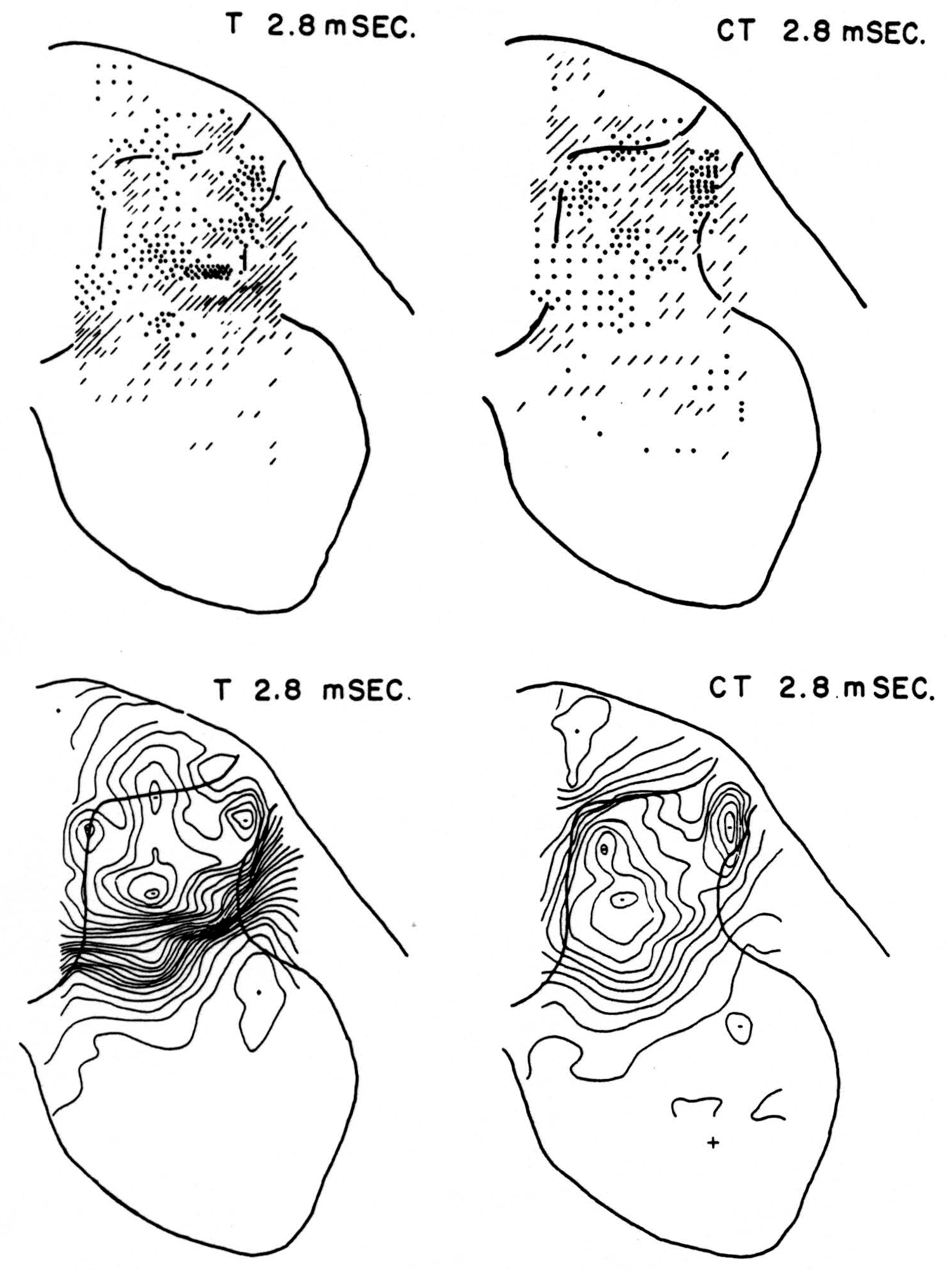
Figure 5. Arranged as in Figs. 3 and 4; top left, source-sink distribution, and bottom left, isopotential map, 2.8 msec. after stimulation of test root alone. Top right, source- sink distribution, and bottom right, isopotential map, at the same time after test root volley but preceded 20 msec. by conditioning volley.
Maps CT after test stimulus to L5 20 msec. subsequent to conditioning stimulus to L6 (Figs. 3-5, CT 1.2, CT 1.6, CT 2.8 msec.)
The sink which had appeared in the dorsal column at 1.2 msec. (T 1.2 msec.), after the test volley alone is almost entirely absent at the corresponding time (CT 1.2 msec.). The residual disturbance set up by the conditioning volley (C 20 msec.) is clearly visible along the dorsal border of the grey matter.
Comparison of maps T, C and CT show that, were the sources and sinks of C subtracted from those of CT, the remainder would be far smaller than the results of T alone. This holds for times 1.2, 1.6, and 2.8 msec. Thus, instead of simple algebraic summation, there is an early interaction which blocks impulses within the white matter of the dorsal column, and consequently there is a much diminished invasion of the grey matter later.
Discussion
There is good general agreement between the distribution of these sources and sinks and those found at approximately the same times in our earlier work with a single stimulating volley (5). The notable differences are the absence of the sink in the ventral horn and a slight difference in the shape and extent of sources and sinks that are a natural consequence of using different animals and different levels in the cord. But the arrangement, order of appearance, and relative magnitudes of the sources and sinks are in satisfactory accord.
It is curious to note that the entering volley arrives at the plane of the electrodes only 1.2 msec. after the stimulus, although its potentials precede it. Our stimulating cathode on the test root lay about 2 cm. away from the cord, and our electrode plane lay about 2 mm. rostral to the rostral edge of the root. Yet up to 1 msec. after the stimulus we measured no activity in the plane. Granting as much as 0.2 msec. utilization time, we can still get no more than 30 m./sec. for the speed of the impulse in the primary afferents. There may be two explanations for this: (i) the very fastest dorsal white matter fibers do not emit collaterals in the plane, and (ii) there exists a region of decrement between root entrance and recording plane. In any case, at T 1.2 msec., the dorsal column sink must represent the earliest arrival of the volley in primary fibers, for there has been no preceding activity up to 1.0 msec., 0.2 msec. is hardly time for adequate synaptic delay, and the distribution of sources and sinks is not that of any known group of internuncials and their processes. Indeed, the subsequent march of the sink along paths taken by primary afferent collaterals in Ramón y Cajàl’s anatomical maps strongly supports such a view. But at this earliest arrival of the volley in the medial white matter, where it has hardly begun to invade the collaterals in the grey at all, it is already greatly reduced by the residual effects of the previous inhibitory volley. The actual site of inhibition, of course, may lie anywhere between the entrance of the test dorsal root into the cord and the medial white matter 2 mm. anterior, where we observe the results. It may be exerted by interaction of parallel fibers or through internuncials; from the present evidence we cannot say which.
Although this study was done under the highly unphysiological conditions which are best for microelectrode maps, we can use its results to suggest more critical experiments. For example, we might be able to see a similar inhibition in the dorsal root rami extending up the dorsal columns to the brain stem. This effect we have confirmed with records from thoracic dorsal column in unanesthetized preparations, and have shown that this inhibition, together with that of the ventral root response and the dorsal root reflex, is increased in magnitude and duration by barbiturates. These findings will be included in a later report.
Principle of Method
As is well known, an action-potential in a fiber recorded in a conducting medium is triphasic—positive as the impulse approaches the electrode, then negative, then positive again as the impulse departs. For this reason, records taken from electrodes in the central nervous system are much worse instruments for localizing activity than records on isolated nerve. The disturbances set up by two impulses are no longer monophasic; and they may cancel one another in any one place as well as add. There is usually a large number of simultaneously active elements in the central nervous system; the potential at any one point is a composite made up of contributions from all active elements everywhere and may reflect principally those at a distance and not those near the recording tip.
These possibilities create much ambiguity in localizing activity from electrical records directly. We therefore seek an index for describing activity in a place which shall be unaffected by fields originating at a distance. We can find one by recalling the description of the nerve impulse in terms of the currents across the surface of the fiber. These likewise exhibit three phases, corresponding to those they contribute to the potential: the part of the fiber ahead of the impulse emits current to the outside; this current flows around and is absorbed by the depolarized segment; the recovering stretch behind the impulse again emits current, which is also absorbed by the depolarized segment. By applying some simple considerations based on the balance of currents to this description, we can obtain an index with the desired properties, and find out how to compute it from measurements of the potential.
In the diagram of Fig. 6, the shaded area represents a depolarized segment of the neurons corresponding to an advancing impulse. Current is therefore passing out of the neurons into the external medium over the unshaded parts, and into them from the medium over the shaded parts, as indicated by the small arrows. Now consider an imaginary box ABCD enclosing part of the cells, and add up the currents crossing the parts of its walls lying in the external medium, counting outward current positive and inward current negative. Currents from elsewhere flowing wholly in the external medium through ABCD do not contribute to this sum: on entering ABCD they count with one sign, on leaving with the other, and the two contributions cancel. Evidently we may write the equation:
net current across walls of ABCD = total current emitted to the external medium by parts of cells in ABCD.
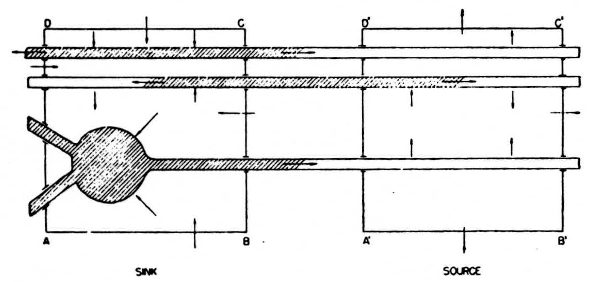
Figure 6. See text.
In the diagram both these currents are inward and therefore, by convention, negative. If we consider a second box A’B’C’D’ enclosing parts of the cells ahead of the impulse, there will be a net outward current across the walls of the box, and this will be equal to the current emitted by the parts of the cells within A’B’C’D’. Again, the net current out of the box is unaffected by currents of external origin passing through A’B’C’D’.
If we imagine the entire region divided up into small boxes of this kind and compute the net current outflow for each such box, it is clear that we shall have the sort of index we are seeking. The net current issuing from the box will be negative when the elements within are active, i.e., are depolarized and absorbing current, and its magnitude will measure the number active; it will be positive when the elements within supply current to other portions of the same cells outside that box. Most important, it is determined only by the state of the elements within the box, in this respect differing from the potential.
We can compute these net currents from the potentials by a rough application of Ohm’s law, as follows. In Fig. 7, E1’, E2’, E3’, E4’ are the potentials on the four sides of ABCD—more precisely, their average values over those sides—and E1, E2, E3, E4 the potentials on four parallel sides at a distance S away. The outward current across CD will be l/SR(E1 —E1’) if R is the specific resistance of the medium, and similarly for the other side. We then find that the net current out of ABCD = (E1’ + E2’ + E3’ + E4’ − E1 − E2 − E3 − E4)
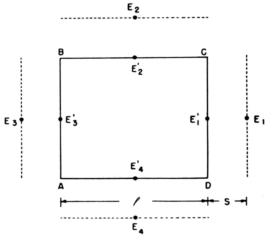
Figure 7. See text.
For a convenient computational expression, consider the dimensions as in Fig. 8. We might estimate the current across CD by the expression
as above, but it is better to use the difference of potentials lying on two sides of CD, namely, E1, and the central value E0, so that the current across CD is
and the net current out of the box ABCD is
This form is useful if the potentials are known for a regularly spaced lattice work of points. As is customary, we shall call this net current j(P0) the source-strength, or source-density, at the central point P0; when it is positive, we say that there is a source at P0; when negative, a sink. The source-density j(P0) is actually the net current issuing from a small volume of size S around P. According to (1), then, we obtain a quantity proportional to j(P0) if we replace each potential in the lattice by the difference between it and the average of its four nearest neighbors. This is the formula we shall adopt for computing.
So far, we have treated the currents as flowing parallel to the plane of the paper. If they do not, the same considerations apply. We shall have to add the current across all six sides of a cubical box; to derive the analogous formula (1) we require the potential to be given at points of a regularly spaced cubical lattice, and then the source-strength j(P0) will be proportional to the potential at P0 minus the mean of the potentials at the six nearest neighbors of P in the lattice.
Discussion of Method
A number of assumptions and limitations are involved in constructing and interpreting source-density maps according to the formula. Some may be justified in part by suitable experimental technique, others can be allowed for to some extent, while all must be borne in mind when extracting and judging conclusions from such maps. It is worth noting that these assumptions are made equally in any other method of tracing impulses through structures by electrical recording; they are no less present, only less apparent, if one does not attempt detailed computation. We shall discuss the principal ones.
I. Mathematically, the derivation of formula (1) is rather crude. To be more precise, let S1 in Fig. 8 be the totality of cell surfaces lying in ABCD, n1 the unit vector directed outward at a point of the cell-surface, S2 the boundary of ABCD, n2 its exterior normal, and R the specific resistance of the external medium. Let E be the potential at points of the external medium: it is convenient to assign it conventionally the value zero at points inside of cells and fibers so that it will be defined everywhere, and we shall not need to exclude the interiors of cells explicitly from the ranges of integration. Then, quite exactly, we have
for j(P), the source-strength at P. For currents parallel to the plane this becomes
To derive the practical formula (1) from (3) requires these assumptions:
- The average values of the potential gradients along ABCD which occur in (3) may be replaced by the values of the potential gradients taken at the mid-points of the sides:
- These derivatives ∂E/∂x at the mid-points of sides are approximately equal to the centered finite differences:
- The resistance R of an external medium changes slowly enough across ABCD to be treated as the same in adding up (4) and (5) to give (1).
Remarks on (i), (ii), and (iii). The purpose of computing source-densities is to cancel out the effects of currents originating outside the volume considered. An approximation to them involves the danger that through-currents, which affect the potential, should contribute to the computed values and produce spurious sources and sinks in the volume. Let us therefore take a case where there are no real sources or sinks and attempt to arrange the lines of current flow so as to violate (i), (ii) or (iii), and give (1) a value significantly larger than zero. If the potential changes linearly along the lines P4P0 and P0P1 in Fig. 8, formula (5) is exact. If it changes parabolically along P4P1, (5) will fail, but the errors in
will be equal, and contribute nothing to (3) or (1). Hence
must change significantly in ABCD and so must
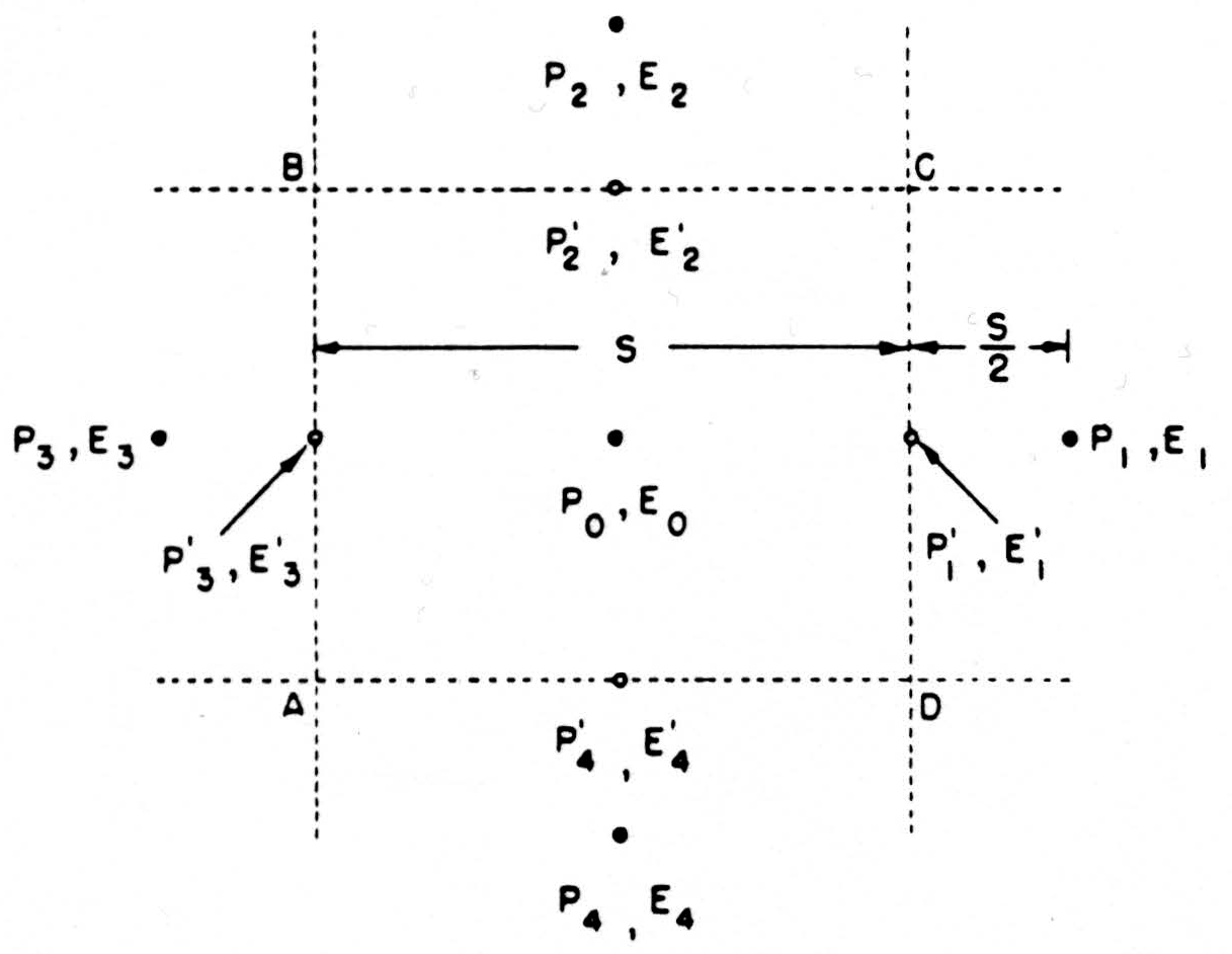
Figure 8. See text.
so that the lines of flow must be quite contorted. It seems likely that this type of flow will happen only where there are obstacles of dimensions that are an appreciable fraction of S, or where there are considerable inhomogeneities in resistance—which amounts to the same thing. When the obstacles are much smaller than ABCD, the current lines will meet around them, with little effect on their general direction.
If variations in the external resistance R are gradual enough to neglect the change over the distance S, (1) will be a valid approximation for each point separately (given (i) and (ii)); in comparing source-strengths at different places, the appropriate value of R will have to be inserted in (1). If R is taken constant, as in our computations, the sources and sinks inside regions of higher resistance (the white matter, perhaps) will come out larger than they ought in relation to the others. They will be correct in sign, nor will any appear where none really is. But if there are two regions V1 and V2 (e.g., white and grey matter within the cord) such that their resistance is nearly uniform within each region, but changes abruptly on the boundary between them, a special consideration applies. Let R1 and R2 be the two resistances, R1 > R2 say, and n the normal from V1 into V2, then
holds on the boundary, expressing the equality of the current across the boundary as measured on the two sides. If one mistakenly assumes a common value R for the resistances of V1 and V2, he will discover a spurious source-density on the boundary whose magnitude per unit area will be
which has the sign of
There will be a spurious source on the boundary where the lines of current flow from a high- resistance region to a low-resistance one, a spurious sink where they are in the opposite direction, each of magnitude proportional to the current density. This criterion is useful in checking the possibility that computed source-densities at such boundaries may be artefacts arising from the sharp change in resistance. If this test is applied to the maps in Figs. 2-5 (as may be done by inspection) at the junction of white and grey matter, then, assuming the white matter has the higher resistance (a 2/1 ratio has been measured (3)) the spurious sources and sinks, if present, would be opposite in sign to those actually found in most places; this applies in particular to the medial part, whence we derive our main conclusion.
It must be remembered that we cannot, in fact, measure the potential at the point P0. What we do is to substitute an inserted conductor for a volume formerly including P0, subjecting it to more or less the same field of sources that formerly created the potential E(P0); it will arrive at a potential determined by the condition that the electrode as a whole must draw no current. The result will be a kind of weighted average of the values of the undisturbed potential for a region whose diameter is usually of the same order of magnitude as that of the recording tip. This helps fulfill assumption (ii). When this assumption fails it is usually because a single element, firing off extremely close to the electrode, so perturbs the recorded potential that it is no longer representative in the sense required by (i) and (ii). Such cases may be recognized from the fact that a very small displacement of the electrode, much less than the normal distance between stations, changes the recorded potential considerably; its shape in time is also quite abnormal. In the spinal cord, with a recording conical tip 10 μ in diameter and about 20 μ long, this happens occasionally, most often in the motor horn, and here it is usually sufficient to advance the electrode halfway to the next station, take a record, and supply the missing value by interpolation; for at that distance the disturbance due to the cell is usually inappreciable. Internuncials and fibers, being about the same size or smaller than the electrode, usually cause less trouble: their discharges are so short and small that the general potential may be traced through them, and they do not often occupy the same positions on repeated records taken from one station.
In favorable conditions, as one moves the recording electrode along its track, he observes a potential wave which changes gradually and regularly with depth, perhaps more rapidly in some regions than in others (See 6, in Fig. 9). In some places a sputter of short spikes appears superposed on the record; they will be of short wavelength, and ordinarily smaller than the potential wave, not interfering with its main outlines, although they may seriously reduce the accuracy of reading. This problem can usually be obviated by taking many records at each place and averaging them, if time permits. Occasionally, a large “cell-spike” may require such procedure. One usually chooses the distance between stations so that intermediate values, when recorded, differ little from values interpolated from those at nearby recording stations.
At this point we may note some considerations determining the optimum size of the recording electrode tip. In the first place, a large electrode engenders mechanical strains on the tissue, which can distort the records; as Lorente de Nó (6) and we (5) have remarked before, the effect is much greater if the electrode is blunt or rough or has a continuously tapering shank, so that it exerts stresses extending to a distance. Moreover, a large electrode tip averages over too large a volume, and limits the attainable resolution. The distance between recording stations must be large compared to the length of the recording tip (in our case, 150 µ as compared to 20 µ or little new information is gained from the intermediate records. On the other hand, if the recording tip is too small, the local perturbations from single active elements nearby increase relative to the general potential, and the error, or “noise,” in the results increases. This may be serious, for the numerical computation has necessarily the unfortunate property of increasing noise relative to the signal. If j is calculated according to the formula
j = 4E0 − E1 − E2 − E3 − E4
from E’s afflicted with independent errors of equal variance σ2, j has a variance 20σ2, so that its probable error is or about 4.4 times that in the measured potentials. Actually, if some of the E’s are calculated by interpolation, the error will be somewhat less, since part of the errors in the E’s will be correlated and tend to cancel out in computing j. In our maps, the random error in j seems to be about three times that in the potentials.
For these reasons we have found no advantage in reducing the electrode tip below 10 µ in diameter. Another reason is that there is little advantage in spacing the recording stations along an electrode track much closer than the distance between neighboring tracks. For obvious technical reasons, it is difficult to reduce this distance appreciably.
It is “noise” which has so far prevented us from making maps under less artificial conditions. Without barbiturates, which reduce the “neural noise” from the background, and without dorsal root stimulation, which provides a larger signal than peripheral nerve, it seems possible to make such maps only by averaging enough records from each station to secure stability.
II. The assumption of planar currents arises entirely for practical reasons: if the potentials are known for a three-dimensional network, the source-density at each point can be computed in an analogous way. The number of electrodes needed would be five, four spaced in a cross about the central one; we could then compute the source-densities along the central electrode. To cover a slice of spinal cord would require about three times the present number of electrodes, and much more labor in interpolating them to a regular lattice. Preliminary measurements showed us that the longitudinal currents in the spinal cord, after a dorsal root volley has already entered the cord, are much smaller than the transverse ones, so that we consider a two-dimensional approximation justified in this case. Moreover, it seems likely that the currents produced by a depolarized fiber should be directed radially from it, in its immediate neighborhood, so that they should contribute to the transverse current-balance, whatever its orientation.
III. The assumption of simultaneity is necessary. In the derivations we have supposed the potentials given everywhere on the network at a fixed instant of time. In fact, they are not: it usually requires two to four hours to insert the electrodes and record from all the stations along each track. We must therefore assume that the record we get from each station is the same we should have seen if we had recorded there at any time during the experiment. This is a difficult assumption to justify with certainty. There are two kinds of events which may upset it. One is a gradual change in the state of preparation during the experiment: this one can minimize by deep anesthesia with a long-acting agent, artificial respiration, strict temperature control ( ±0.1°), constant suffusion of the mineral oil with O2 and CO2 in proper concentration, and the use of supramaximal stimuli. The other is a possible change produced by the recording procedure itself. One can monitor such changes by watching various functions of activity in the cord: the dorsal root potentials, the ventral root potentials, and perhaps the surface potentials. In addition, one ought to watch the pial circulation on the dorsum through the microscope used to check the insertion of electrodes. If all these things remain constant during the experiment, there are reasonable grounds for treating the measurements as if they were contemporary. Naturally, it is only under special conditions, in special structures, that such procedures are permissible. We feel more confidence in this assumption since finding that our maps are reproducible independent of the order of inserting the electrodes.
IV. Since our electrode tracks are never quite parallel or evenly spaced, we must derive regularly spaced values from them by interpolation. When the observed values are spaced about as closely as the regularly spaced interpolated ones which replace them, the procedure does not need much justification. If there is a gap in the observations as in the center of Fig. 1 (because of the discarded electrode track), interpolation may lead to more error, and the distribution of source-strengths in that region is less reliable in detail than on both sides of it. It is worth remarking that linear interpolation between observed values cannot be used, for it is equivalent to assuming the source-strengths entirely concentrated at datum points, with vanishing source-density between. Numerical interpolation must employ second differences at least; we have found that taking account of higher differences introduces too much random error to be useful. In principle, it would be best to use true two-dimensional interpolation by Newton’s divided differences, but this is too laborious. We therefore interpolate along the electrode tracks to reach values at their intersections with horizontal lines on graph paper—this is easy because the datum values are equally spaced—and then interpolate by second divided differences along the horizontal lines to reach values at each node. Replacing Newton’s method by successive one-dimensional interpolations probably contributes to the frequency of horizontal and vertical lines as boundaries of source and sink regions, although much of that appearance in the diagrams comes from the method of drawing them.
We have likewise tried graphical interpolation instead of the lengthy numerical method. The result is a map of source-densities of the same general character as the other, but rougher, and with a few significant differences in detail. This may happen because two different “smooth” curves drawn through the same points by different people will generally differ more in curvature than in height at a place, and it is curvature that contributes to the source-densities. In general, graphical interpolation gives only a reasonable first approximation.
V. If a volume is selected that is large enough to contain a cell and all of its processes, that cell will contribute nothing to the net current from the volume, since the total current flowing out of a cell is exactly equal to that flowing into it elsewhere. For axons, as Erlanger and Gasser have pointed out, the duration of the depolarized region in time is not far from 1 msec., independent of size of fiber; this would make its length in millimeters numerically equal to the conduction velocity in meters per sec. For a 100 m./sec. fiber this is 10 cm.; for a 1 m./sec. collateral, 1 mm. With a grid whose spacing is 150 µ, it is possible that active internuncials of short axon should fail to show up, but unlikely that collateral fibers should. Enough temporal dispersion in a volley can produce some cancellation; in any case, the sinks are likely to dominate, being much more intense than the source on any single part of the same cell. The dispersion can be reduced by using supramaximal stimuli. Again, electrotonic currents in neighboring elements will reduce the apparent strength of sources and sinks arising from depolarized cells, but it does not seem likely that so much of the action current would flow into neighboring fibers, so little through the external medium, as to conceal the activity entirely—except perhaps in the dorsal root ganglion, according to Svaetichen (7).
Conclusion and Summary
Dorsal roots L6 and L5 were stimulated in such a way that a volley in one inhibited the motor response to a volley in the other. With multiple microelectrode placements, we measured the potential changes and calculated the current distribution in a cross section of the cord traversed by these dorsal root fibers. We were thereby able to follow the intramedullary course of afferent impulses. It was shown that, after stimulus of L6, test volleys in L5 failed to invade collaterals of the primary axons. We conclude that one type of inhibition involves blocking afferent nerve impulses before they have reached the region of cells.
Footnotes
Acknowledgment
We want to thank the computing group, under Miss Elizabeth Campbell (Mrs. Hannah Wasserman and Miss Gloria Freedman, in particular), for performing the tedious computations involved in this work.
References
Ballif, L., Fulton, J. F., and Liddell, E. G. T. Observations on spinal and decerebrate knee jerks with special reference to their inhibition by single break shocks. Proc. Roy. Soc., 1925, B98: 589-607.
Barron, D. H. and Matthews, B. H. C. The interpretation of potential changes in the spinal cord. J. Physiol., 1938, 92: 276-321.
Renshaw, B. Observations on interaction of nerve impulses in the grey matter and on the nature of central inhibition. Amer. J. Physiol., 1946, 146: 443-448.
Eccles, J. C. and Malcolm, J. L. Dorsal root potentials of the spinal cord. J. Neurophysiol., 1946, 9: 139-160.
Pitts, W. Investigations on synaptic transmission. Cybernetics, Trans. 9th Conf., 1952: 159-166.
Lorente De Nó, R. Action potential of the motoneurons of the hypoglossus nucleus. J. cell. comp. Physiol., 1947, 29: 207-287. ’
Svaetichen, G. Analysis of action potentials from single spinal ganglion cells. Acta physiol, scand., 1951, 24: 23-55.
Crile, G. W., Hosmer, Helen R., and Rowland, Amy F. The electrical conductivity of animal tissues under normal and pathological conditions. Amer. J. Physiol., 1922, 60: 59-106.
Epi-search analysis
Word cloud:
Activity, Alone, Along, Cells, Changes, Compute, Conditioning, Contribute, Cord, Current, Differences, Distance, Distribution, Dorsal, Electrode, Error, Fibers, Figure, Flow, Frac, Grey, Impulses, Inhibition, Interpolation, Lines, Maps, Matter, Measured, Medium, Msec, Net, Partial, Plane, Points, Potential, Recording, Region, Resistance, Root, Sinks, Source-Density, Sources, Spinal, Stations, Stimulation, Test, Values, Volley, White.
Topics:
Sources, Current, Interaction, Maps, Electrodes, Record, Currents, Changes
Keywords:
(final) Experiment, Microelectrodes, Al, Use, Inhibition, Root, Maps, Wiring, Nerve, L7
(full text 1) Frac, Stimulation, Dorsal, Cord, Inhibition, Potentials, Neurons, Root, Lattice, Electrode
(full text 2) Interaction, Root, Microelectrodes, Inhibition, Maps, Use, Experiment, Response, Nerve, L6
Citations:
Related Articles:
Related books:
Keywords from the citations and related material:
Cortex, Brain, Stimulation, Neurology, Physiology, Responses, Stem, Lobe, Monkey, Projections