Systems theory and complexity:
Part 3
Kurt A. Richardson
ISCE Research, USA
Introduction
In previous installments of this series (Richardson, 2004a, 2004b) I have explored a number of general systems theory laws and principles from a complex systems perspective. One of my key motivations for this is to understand (albeit in a limited way) the relationship between systems theory and its more recent incarnation, complexity theory. For those readers who have not yet read parts 1 and 2, the following laws/principles have thus far been considered:
- 2nd law of thermodynamics (part 1);
- complementary law (part 1);
- system holism principle (part 1);
- darkness principle (part 1);
- eighty-twenty principle (part 1);
- law of requisite variety (part 2);
- hierarchy principle (part 2);
- redundancy of resources principle (part 2), and;
- high-flux principle (part 2).
In part 3 I will explore six more systems principles from the perspective of complexity. As previously I will use relatively ‘simple’ Boolean networks to illustrate the main points where possible. In the next issue (part 4) I will explore how the general systems movement evolved in an attempt to appreciate how the complex systems movement might develop. As such I will move away from considering specific laws and principles. In total fifteen laws/principles would have been explored, all of which I have taken from Skyttner’s (2001) General systems theory. In that book a total of forty-three general systems laws/principles/theorems are listed―far too many to consider in this series. I have added an appendix to this installment listing those not discussed and I encourage the interested reader to consult Skyttner, (2001) for further details.
Sub-optimization principle
Skyttner (2001: 93) defines the sub-optimization principle as follows: “If each subsystem, regarded separately, is made to operate with maximum efficiency, the system as a whole will not operate with utmost efficiency.”
We can also add the reverse: if the whole is made to operate with maximum efficiency, the
comprising subsystems will not operate with utmost efficiency. Another way to think about this is simply to acknowledge that parts in isolation behave differently from parts that are connected to an ‘environment’. I’d like to illustrate this principle through a Boolean network of networks.
Figure 1 shows a relatively simple network of sub-networks. Each sub-network (or sub-system) contains ten interconnected nodes that operate on fixed nonlinear rules (the full details have been omitted but are available on request). Each sub-network has one outgoing and one incoming connection to each of the other three sub-networks. As such the ‘environment’ for each sub-network is itself a network of sub-networks. Once functional rules have been selected for each node, it is a relatively simple matter to then construct the phase maps for each sub-network and the network of sub-networks as a whole. In the realm of Boolean networks we say that the network’s function is characterized by the number and period of its phase space attractors. For example, if we consider sub-network 1 (St) in isolation (i.e., remove its connections to the other subnetworks) we find that its phase space is characterized as 3p4 which means that its phase space contains three period-four attractors, or that trajectories from each point in phase space will eventually (assuming no external interference) fall onto one of three possible attractors. In the case of genetic regulatory networks, each different attractor represents a different cell type. Table 1 lists the phase space structure and topological structure (i.e., the structural loops that result from the inter-nodal connections) for each of the sub-networks comprising Figure 1. The phase/topological structure for the overall network of sub-networks (S1234) is also included.
To illustrate the sub-optimization principle we need to ‘optimize’ the networks. We can do this from at least two directions: from the bottom-up and from the top-down. The optimization of Boolean networks is achieved by removing those nodes and connections that do not contribute to the network’s function, i.e., those that do not affect the gross qualitative structure of phase space. The optimized network will still have the same phase space characterization, but may contain (significantly) fewer nodes and connections. This process was discussed in Part 1 under the ‘eight-twenty principle’ and is explored in full detail in Richardson, (2005). The bottom-up optimization process begins with the optimization of each sub-network in isolation from the network of sub-networks as a whole. Once optimized the original connections between each sub-network are added (where the original node still exists) and the phase space of the resulting (bottom-up optimized) network of sub-networks (shown in Figure 3) is examined.

Figure 1 An example of a Boolean network of sub-networks showing inter-nodal and inter-sub-network connections. Nodes with a circle around them also contain a connection to themselves.
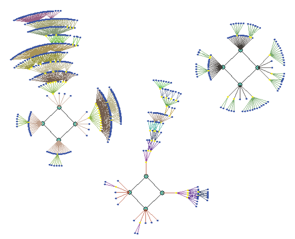
Figure 2 Attractor basins for sub-network S1. The attractor space is characterized by three period-four attractors.
| Sub-network | Phase space, p, structure | Structural feedback, P, loops |
| S1 | 3p4 | 3P1,3P2, 2P3,1P4, 1P6 |
| S2 | 2p1,1p2 | 2P1, 3P2, 3P3, 4P4,2P5 |
| S3 | 4p2, 2p4 | 3P1,1P2,1P3, 2P4,1P5 |
| S4 | 3p1, 1p2, 2p3 | 3P2,1P3, 3P4, 5P5, 4P6,1P7,1P8, 1P9 |
| S 1234 | 4p4, 2p8, 1p52,1p76 | 8P1,10P2, 8P3,10P4, 9P5, 5P6, 6P7, 8P8, 9P9, 5P10,12P11, 15P12,8P13,12P14, 10P15,11P16,10P17, 3P18,3P19, 2P20 |
Table 1 Sub-network and ‘network of sub-networks’ characteristics.
Table 2 lists both the phase space and topological structure for each of the optimized sub-networks and the network of sub-networks as a whole. The first thing to note is that the (bottom-up) optimized networks contain considerably fewer (structural) feedback loops. The most important point, however, is that the phase space structure for the overall network of sub-networks in now quite different from what it was before. By optimizing the sub-networks the behavior of the network of sub-networks has changed considerably. If we were to top-down optimize the resulting network (via the method described shortly) we would also find that the network of sub-networks was not optimized, i.e., local optimization does not (necessarily) lead to global optimization. Further more, optimizing the function of the parts changes the functional behavior of the whole (shown by the change in its phase space structure).
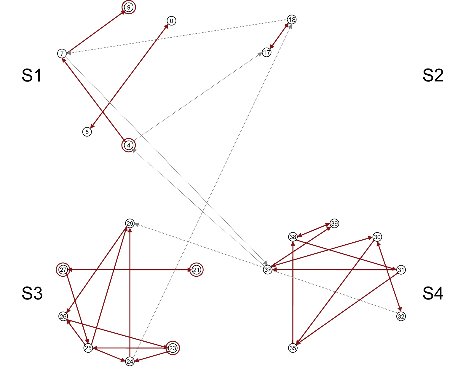
Figure 3 The bottom-up optimized version of the ‘network of sub-networks’ shown in Figure 1.
| Sub-network | Phase space, p, structure | Structural feedback, P, loops |
|---|---|---|
| S1 | 3p4 | 2P1,1P2 |
| S2 | 2p1,1p2 | 1P2 |
| S3 | 4p2, 2p4 | 3P1,1P2,1P3, 2P4, 1P5 |
| S4 | 3p1, 1p2, 2p3 | 3P2,1P3,1P4, 1P5 |
| S1234 | 1p4, 8p8, 2p12,1p28, 8p56,2p84 | 5P1, 6P2, 3P3, 3P4, 3P5,1P9, 1P10 |
Table 2 Sub-network and ‘network of subnetworks’ characteristics of the bottom-up optimized system
We can also approach optimization from the top-down. Here we optimize the network of sub-networks as a whole and then isolate what’s left of the constituent sub-networks so that their individual behavior can be determined. So the top-down approach identifies which nodes and connections do not contribute to the overall functionality of the network of sub-networks rather than the functionality of each sub-network. The resulting top-down optimized network of sub-networks, which is shown in Figure 4, has (qualitatively) exactly the same phase space structure as the initial network of subnetworks shown in Figure 1. However the phase space and topological structure of the component sub-networks has changed (although in two cases―S2 and S3―the phase space structure is actually the same, but the sub-networks themselves are not optimized). Table 4 contains the relevant data.
This short analysis of a Boolean ‘network of sub-networks’ illustrates two important points:
- optimization of a system’s parts does not (necessarily) lead to an optimal system, and vice versa;
- optimization of a system’s parts, although not changing the functionality of those same parts, can change the functionality of the system as a whole and vice versa.
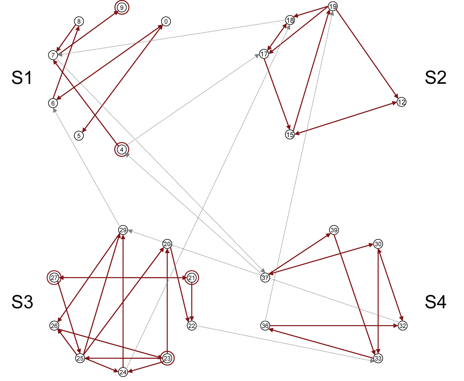
Figure 4 The top-down optimized version of the ‘network of sub-networks’ shown in Figure 1.
| Sub-network | Phase space, p, structure | Structural feedback, P, loops |
|---|---|---|
| S1 | 2p4 | 2P1, 2P2 |
| S2 | 2p1,1p2 | 2P2, 2P3,1P4 |
| S3 | 4p2, 2p4 | 3P1,1P2,1P3, 2P4, 1P5 |
| S4 | 1p1 | 2P2,1P4,1P6 |
| S1234 | 4p4, 2p8, 1p52,1p76 | 5P1,7P2,4P3,4P4, 2P5,1P6,4P7, 3P8, 4P9,1P10, 2P11, 2P12,1P13, 2P14, 1P15 |
| Table 3 Sub-network and ‘network of subnetworks’ characteristics of the bottom-up optimized system. |
This consequence of systemic, networked, behavior poses some interesting challenges for the designers and managers of human organizations. The notion of an organization being efficient at all levels and across the board would seem to be an impossibility. Efficiency (which I am regarding here as the direct consequence of optimization) in some areas will lead to lower levels of efficiency in other areas. Treating the organization as a ‘whole ’ as some holistic thinkers would have us do does not address this issue adequately either. Considering what would be ‘best’ for the whole may not be (I am almost prepared to say “will not be”) ‘best’ for the component systems (parts) that comprise the whole. In principle only some functions can be optimized, not all. Although in practice, given the overwhelming complexity of huge numbers of interacting sub-networks (many of which we can’t even write down a close, let along complete, representation of), optimization at any level is an ideal we can never fully realize.
A last comment on the sub-optimization principle: in order to optimize the sub-networks in the bottom-up approach the individual sub-networks had to be considered in isolation. Although it was shown that when connected to their ‘environment’ the net resulting behavior was different, the behavior of those same (bottom-up optimized) sub-networks ‘in connection’ rather than ‘in isolation’ was not really examined. I like to explore this difference a little before moving on to the next principle.
By isolating the sub-networks we are closing them; they are no longer open. As such, once the sub-network is moving along a particular trajectory, it will converge on a particular attractor and it will then cycle through a fixed number of states in the same order forever more. The system certainly can not move from one attractor to another. However, once the sub-network is connected to an ‘environment’ rather more complex behaviors can occur. For example, signals from outside the system can push it towards a different attractor. Furthermore, new attractor hybrids become available through the interaction with the ‘outside world’ as ‘information’ flows through longer period feedback loops, and as more loops interact with each other in non-trivial ways.
To illustrate this consider Figure 5. The top (Figure 5a) shows the asymptotic behavior (i.e., steady state behavior with transients removed) of the isolated sub-network S4―three period-1, one period-3 and three period-2 trajectories are shown. Notice that the periods are relatively short (compared to network size, N=10), and that each trajectory appears quite ‘pure ’ in that they do not seem to be combinations of other trajectory types (although both the period-three trajectories might be regarded as period-two trajectories if transformed to a different timescale). Another important point is that within a particular cycle each state is unique, i.e., you won’t observe a period three attractor containing repeated states like 955, 955, 345. For every state in phase space there is only one possible next step (whereas in this particular example it seems that the next step from 995 can, at least, be either 955 or 345―the next state is not uniquely defined).
Figure 5 The different (steady-state) trajectories for sub-network S4 (a) ‘in isolation’, and (b) ‘in connection’. Note that for (b) each series has been offset for clarity.
The case for S4in vivo is quite different indeed. Other than the p2 (period-two) trajectory (which is the attractor the sub-network follows for all the four period-4 attractors exhibited by the overall network of sub- systems), all the attractors seem to be ‘hybrids’ of other types. For example, the top most p8 trajectory seems to be a hybrid of a p1 trajectory (the flat line) and a p4 (which is nearly a p2) trajectory, i.e., the system intermittently jumps from a p1 attractor to a p4 (or a p2 repeating twice) attractor (resulting in a period-eight cycle overall). This is the result of external signals (from the rest of the network of sub-networks) forcing the sub-network to jump between (at least) two different attractors. The word ‘forcing’ here is a little misleading because the existence of the S4 sub-network within the network of sub-networks partly account for this p8 attractor in the first place―signals from the sub-system into the larger ‘environment’ contribute to the ‘emergence’ of the particular phase space structure that the overall network of sub-networks exhibits. What we would tend to expect is that the ‘environment’ is harder to ‘perturb’ than the sub-network.
Another important feature to note from this particular intermittent behavior is that during the flat-line (p1) period three exact same states repeat (the fourth is actually a slightly different state), before the shift to a different sequence. As indicated above, this would never occur in the isolated (in vitro) sub-network.
The second p8 attractor looks a little like a distorted p2 and the two long period (compared to the sub-network size) look like the sub-system is being externally disturbed so frequently that it is unable to settle down to a stable mode of behavior―in one time step the sub-network follows a p2 attractor and in the next time step it follows a p8 attractor, say; never having time to ‘find its feet’. What results appears to be random behavior, despite the very ordered structure of the overall network of sub-networks’ phase space. In short, in isolation (in vitro) the S4 sub-network’s phase space is described by 3p1, 1p2, 2p3, whereas in connection (in vivo) the same sub-network’s phase space might be described as:
- one period-two attractor;
- one intermittent period-two attractor;
- one distorted period-two attractor, and;
- two different ‘quasi-random’ attractors.
My point here is simply that the ‘in isolation’ and ‘in connection’ behaviors are very different indeed. In a sense this is the principal distinction between the natural sciences and the social sciences. On the one hand, the natural sciences focus on objects ‘in isolation’ (and fortunately many of the objects of natural science can actually be usefully examined ‘in isolation’). Whereas, on the other hand, the social sciences attempt to comprehend objects that cannot easily be isolated, and when ‘connected’ objects are effectively isolated (‘disconnected’) they behave very differently indeed. More recently the natural sciences have taken an interest in ‘connected’ objects, in say ecology for example, and we are beginning to appreciate how distorted our understanding of open systems is when we are essentially forced to reduce them to a closed description for the purposes of analysis. The short analysis provided above illustrates how the gap between what we are able to determine and what actually is can be very wide indeed.
Redundancy of potential command principle
This principle is closely related to the darkness principle that was discussed in part 1, in that there are limits to our representations of complex systems. Skyttner (2001: 93) defines the redundancy of potential command principle as follows:
“In any complex decision network, the potential to act effectively is conferred by an adequate concatenation of information.”
Essentially this means that to ‘control’ a complex system we must at first have a sufficiently good representation of it, so that we can design our controlling actions such that our desired effects will follow as a direct consequence. The task of constructing such a “sufficiently good representation” is problematic when we are concerned with complex systems. Part of the reason for this is that any repre-sentation is by necessity an abstraction, and abstractions are incomplete. Such incompleteness always leaves open the possibility, because of sensitivity to initial conditions (context), that our basis for taking action might be (sometimes wildly) inaccurate. This is true even if the ‘real’ system is a closed system―slightly incomplete descriptions do not necessarily lead to slightly incomplete understanding. A related reason results from the fact that even if the description of the open system itself is complete (which is rarely the case anyway), it is practically impossible to have a complete description of the environment within which the open system of interest operates. There are analytical strategies for mitigating the consequences of limited representations/models/ abstractions (e.g., sensitivity analysis, triangulation, etc.), but more often than not there is no way to fully account for the possible disturbances from outside the system of interest and how they might affect it.
Effective control relies on effective prediction and complexity writers often focus on the limitations imposed on effective prediction by chaos (i.e., sensitivity to initial conditions). Indeed, if all systems of interest behaved chaotically then there would be very severe limitations on our ability to make effective prediction (although certain types of prediction―such as qualitative predictions―can be made quite effective). However, complex systems also exhibit, anti-chaos, or, as it is more usually labeled, self-organization. The forces of chaos and anti-chaos engage each other leading to contexts for which effective prediction is impossible, and to contexts for which effective prediction is a very straightforward matter. Most ‘real’ contexts exist somewhere between these two extremes and so all we can really say at the general level is that effective prediction within complex systems is problematic and context dependent (rather than impossible).
Effective prediction can be linked to our ability to extract meaningful (or effective) patterns from the data available. If the patterns we observe are very ordered then creating an abstraction that is not too far removed from reality is relatively straightforward. Furthermore, given a choice of abstractions, we can make a good assessment as to which one is the ‘best’. We say that ordered patterns are highly compressible. On the other hand, if the patterns we observe are purely random (i.e., not chaotic as chaotic patterns are simply a disguise for some underlying order), then there is no adequate abstraction that would capture the essence of the pattern. Alternatively, we could also that there are an infinite number of possible abstractions, none of which could be selected over any of the others (in a way, saying that there is no discernible pattern is the same as saying that there is an infinite number of discernible patterns―neither situation facilitates the generation of understanding). Contrary to ordered patterns, random patterns are wholly incompressible. There is a middle ground between the ordered and the random, which is sometimes called the complex, in which the patterns are neither compressible or incompressible in any absolute sense. Figure 6 attempts to illustrate this middle ground.
Figure 6a shows an example of an ordered patterns that is highly compressible, whereas Figure 6c shows a random pattern which is incompressible, i.e., the shortest representation of the pattern is the pattern itself. Figure 6b illustrates the middle ground with a complex pattern. If we were to demand a complete representation then the shortest representation would be the pattern itself. In this sense the complex pattern is indeed incompressible, which might lead one to think that it is random (or at least chaotic). However, the lower half of Figure 6b shows a plausible compression of the pattern which captures its essential features. Although the compression shown is incomplete it will prove meaningful, i.e., useful, for certain purposes. Using the language above, the lower figure provides “an adequate concatenation of information.”
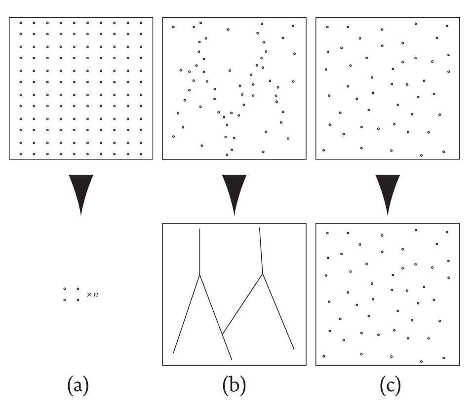
Figure 6 The distinction between (a) ordered, (b) complex and (c) random patterns in terms of their compressibility.
In an absolute sense, complex patterns are indeed incompressible, but at the same time they are quasi-compressible. In this sense, effective command requires effective compression, but because the compression is incomplete such command is necessarily fallible. Whereas for random patterns, we might say that all compressions are equally valid (or, equally ‘bad’), for complex patterns, although there may be more than one meaningful compression, some compressions are better than others and effective command (and control) starts with a consideration of multiple meaningful compressions (where the determination of ‘meaningful’ contains a not insignificant subjective element).
Relaxation time principle
The relaxation time principle states that “system stability is possible only if the system’s relaxation time is shorter than the mean time between disturbances” (Skyttner, 2001: 93). The basis of this particular principle was hinted at in the above discussion of the sub-optimization principle when the effect of external signals on ‘in connection’ systems was briefly explored. I asserted that the long period attractors (p52 and p76) shown at the bottom of Figure 5 were the result of frequent external signals pushing the sub-network into different attractors so often that the sub-network could not settle onto one particular attractor for any significant length of time.
The notion of a characteristic relaxation time is also hinted at in Figure 2 where three attractor basins are shown. Note that surrounding each attractor (the squares at the middle of each basin) are branches of state transitions that all end on one of the attractor states (before then cycling around all the attractor states). If we consider the left hand side attractor basin in Figure 2 we can see that the furthest states from the central attractor are a maximum of ten steps away, i.e., if the sub-network is initiated from one of these states it will be ten time steps before the sub-network settles, or relaxes, onto its period-four attractor. By considering all the branches of non-attractor states we could easily calculate the average number of steps that all the points in phase space are away from the central attractors―this average number of steps is called the average relaxation time. These branches are sometimes called transient trajectories (or nonsteady state). So, for any complex system that is initiated from a certain set of conditions, or is pushed into a certain set of conditions from external factors, there is a transient delay before the system will reach it characteristic attractor. In some instances the relaxation time can be so long that an observed system may not actually reach a phase space attractor during the observation period. This is problematic in that some systems may appear to be chaotic, or even random, because of very long disorderly transients, even though after a sufficiently long time the system might settle onto a very simple attractor cycle.
Given that there is often a delay between any transient state reaching an attractor state, it seems obvious that if the time between external disturbances is shorter than the relaxation time on average then the system will rarely get the chance to settle down in to its characteristic behavior. As such the observed behavior might appear very disordered despite the natural tendency of the system to seek out an orderly behavior. I say “it seems obvious” because not all external disturbances will lead to such significant effects (as pushing the system into another attractor basin). For example, if the system’s phase space is characterized by a single long-period attractor then there is a greater chance that an external perturbation will push the system from one point on that attractor to another point on the same attractor, rather than on to a point on one of the attractor basin branches (after which a delay would follow before the attractor was reached again). In this scenario, although the system’s behavior is disrupted, the system immediately recover’ (i.e., the local relaxation time is zero).
It should also be noted that if signals from within can destabilize the system as well. This suggests that if management attempts to change an organization too often then the organization may not be given the chance to ‘work through’ the previous changes and make the best of them. New changes may be made to an organization already in transition, which would make it more difficult to actually determine what changes may be useful. There has been a lot of focus on organizational change lately; maybe it’s time to reconsider the positive benefits of organizational inertia rather than seeing it as an obstacle to change.
Negative/positive feedback causality principle
One of the motivations for beginning this series was to point out that a number of the ideas and concepts that are often seen as having been introduced recently by complexity theorists were in fact known to early general systems theorists. A good example of this is the feedback causality principle which has both negative and positive modes.
The negative feedback causality principle says that:
“Given negative feedback, a system’s equilibrium state in invariant over a wide range of initial conditions” (Skyttner, 2001: 93).
This characteristic is also known as equifinality, and basically suggests that a system’s phase space contains basins of attraction. The term “system’s equilibrium state” should not be confused with systems in which there is no change at all. The equilibrium state of a chaotic system is a state in which the system trajectory follows a chaotic (strange) attractor. Negative feedback is the mechanism by which phase space is carved-up into different regions of attraction, i.e., rather than all states being equally likely (as in thermodynamical systems) certain states are more likely than others and those states lie on attractors. The branches that feed into the attractors in Figure 2 contain the “wide range of initial conditions” all of which eventually end up on the same attractor; many different starting points end up in the same place; or, there are many ways to achieve the same ends. This contains both ‘good’ and ‘bad’ news for the managers of complex organizations. On the one hand, there are many ways for a manager to achieve the same desired goals. On the other hand, there are many ways for the same system to achieve a goal that is different to the one desired by the manager. When interacting with complex systems, it seems that we will always have to take the ‘bad’ with the ‘good’―a ‘1st law of complexity’ perhaps!
Equifinality ensures that many starting points will take us to the same end point. Multifinality (or the positive feedback causality principle) ensures that the same starting point will lead us to many different end points. Again, even relatively Boolean networks provide an adequate framework for thinking about multifinality. If we consider a small Boolean sub-network (which remember is a deterministic system) and include a source of random external perturbations then, if the system is initialized in exactly the same way over multiple model runs, it is possible for the system to be in any one of the attractors that characterize that system’s phase space. In other words, from the same start point, qualitatively different end points can be reached. Of course, in this simple example, the number of different possibilities is exactly the number of attractors available. Furthermore, the source of ‘creativity’ that allows the system to explore these different possibilities comes from outside the system; there is no internal mechanism that would allow the system to ‘jump attractors’ (i.e., cross separatrices, or bifurcate). In complex (adaptive) systems, however, both external and internal ‘perturbations’ can provide a source for attractor ‘jumping’. Moreover, in such systems the structure of phase space can evolve which, will change the number of nature of the available attractors. Whereas in the complex (Boolean) system the set of attractors (available endpoints) is pre-determined―which means that in principle any of the other end points could be reached from the current end point―the set of attractors for a complex adaptive system can evolve over time (the system actually becomes a different system from that which it started). As such the same initial conditions can evolve into different systems with different phase spaces. In this instance, moving from a particular end point (attractor) in one phase space to a particular end point in another phase space would only be achievable only through radical reconstruction of the system itself.
Again, this characteristic contains both ‘good’ and ‘bad’ news for managers. On the one hand, in an applied research (problem-solving) scenario several teams might be equipped with the same resources and yet a range of different ‘solutions’ might be found by those teams; multifinality might be regarded as the ‘ 1st law of creativity’. On the other hand, the same managerial strategy will lead to a range of different outcomes, some of which may not be desirable; all creativity is not necessarily good.
The patchiness principle
The idea of the ‘edge of chaos’ would, for many complexity thinkers, be a good candidate for an idea unique to modern complexity theory. Once again a similar notion can be found in general systems theory.
To be honest it is not obvious to me what the ‘edge of chaos’ means as it has been used in so many ways. In the area of Boolean networks the ‘edge of chaos’ refers to those networks whose behavior is neither ordered or quasi-random, but complex (like the examples given in Figure 6). This is achieved in such networks by the emergence of non-interacting modules that together limit the overall behavior of the network (Bastolla & Parisi, 1998; discussed briefly in part 2 of this series). In quasi-random networks modularity is absent and so very large (relative to network size) attractor cycles are possible. Ordered networks contain only non-interacting (linear) feedback loops whose individual behavior is easily understood as is their nett behavior (as they do not interact). Behaviorally complex Boolean networks occupy the middle ground where non-interacting sub-systems exist. Here, ‘walls of constancy’ emerge that limit the flow of information throughout the network and therefore restrict the overall behavior. It is a balancing act between mechanisms that facilitate the flow of information and mechanisms that prevent such flows.
Although the term ‘edge of chaos’ has been used in different ways, it always seems to indicate a balancing act between two extremes. For example, in application to human organizations, the ‘edge of chaos’ has been used to describe the balancing act between the need to perform core activities (i.e., those activities that currently generate profit―sometimes equated with ‘ordered’ rule-based behavior) efficiently, but at the same time invest in ‘blue sky’ activities (sometimes equated with ‘chaotic’ behavior―wrongly in my opinion) to ensure that core activities change with changing customer needs. Although this application of the ‘edge of chaos’ is quite different from the one above, the importance of maintaining a balance between two extremes is common to both. This maintenance of some kind of balance is central to the patchiness principle.
Skyttner (2001: 95) describes the patchiness principle as follows:
“The lack of capacity to use a variety of resources leads to instability... Rule-bound systems, stipulating in advance the permissible and the impermissible, are likely to be less stable than those that develop pell-mell.”
So, to maintain a level of stability in the face of changing conditions a system should not invest too much time and effort into one particular way of doing things. A capacity to take advantage of a plurality of resources allows the system to ‘move with the times’―this is the essence of the ‘edge of chaos’ and illustrates once again the strong connections between general systems theory and modern complexity theory.
Moving on from GST
Tus far in this series I have equated the systems movement mainly with general systems theory. In a sense much of modern complexity theory is a direct development of general systems theory with its focus on mathematical means for exploring systems-based behavior; general systems theory with powerful computers, if you like. However, complexity theory is only part of a larger complexity movement that we might call ‘complexity thinking’ or ‘complexity studies’. Although the mathematical understanding of complexity continues to provide new insights, some complexity writers are developing in other directions partly in response to the growing awareness of the limitations of formal mathematical representations. For example, David Snowden, (2002) with his keen interest in the role that narrative and metaphor plays in the sense making process, or Paul Cilliers, (2000) with his concern with the limits to our understanding and the essential role that ethics must play in our comprehension of complex systems. I could name many more. Complexity theory is evolving in different directions, some of which would not traditionally be considered as science. Because of this move away from rigorous mathematical analysis certain directions are seen as ‘not science’ in some circles and therefore are not legitimate paths to tread in our journey to understand complexity to our best abilities. The emergence of these different threads will not be new to veteran systems thinkers. General systems theory evolved and bifurcated allowing quite different systems ‘paradigms’ to emerge, such as soft systems thinking, critical systems heuristics, boundary critique, etc. Systems theory can no longer be equated with the general systems movement of the mid-19th Century as it often is. Given that the different complexity ‘paradigms’ seem to be developing in a way very similar to how general systems theory branched-out, the next episode will provide a short analysis of the systems movement and how it has developed over the past 50 years. I hope that in doing so we might better understand the current state of complexity thinking and its developmental possibilities, as well as encourage renewed collaboration between the two broad communities.
Appendix 1 Further systems laws, principles and theorems presented in Skyttner, (2001)
- The law of requisite hierarchy;
- The law of requisite parsimony;
- Homeostasis principle;
- Steady-state principle;
- Viability principle;
- First cybernetic control principle;
- Second cybernetic control principle;
- Third cybernetic control principle;
- The feedback principle;
- The maximum power principle;
- The omnivory principle;
- The variety-adaptability principle;
- The flatness principle;
- The system separability principle;
- The redundancy principle;
- The buffering principle;
- The robustness principle;
- The environment-modification principle;
- The over-specialization principle;
- The safe environment principle;
- The principle of adaptation;
- Godel’s incompleteness theorem;
- Redundancy-of-information theorem;
- Recursive-system theorem;
- Feedback dominance theorem, and;
- Conant-Ashby theorem.
References
Bastolla, U. and Parisi, G. (1998). “The modular structure of Kauffman networks,” Physica D, ISSN ,115: 219233.
Cilliers, P. (2000). “Knowledge, complexity, and understanding,” Emergence, ISSN 1521-3250, 2(4): 7-13.
Richardson, K. A. (2004a). “Systems theory and complexity: Part 1,” Emergence: Complexity & Organization, ISSN 1521-3250, 6(3): 75-79.
Richardson, K. A. (2004b). “Systems theory and complexity: Part 2,” Emergence: Complexity & Organization, ISSN 1521-3250, 6(4): 77-82.
Richardson, K. A. (2005). “Simplifying boolean networks,” accepted for publication in Advances in Complex Systems, ISSN 0219-5259.
Skyttner, L. (2001). General systems theory: Ideas and applications, River Edge, NJ: World Scientific, ISBN 9810241755.
Snowden, D. (2002). Using narrative in organizational change, Collaboration, ISBN 1901457036.