Introduction
Understanding the structure of complex networks and uncovering the properties of their constituents has been, for many decades, at the center of study of several fundamental sciences, such as discrete mathematics and graph theory. In the past decade there has been an explosion of interest in complex network data, especially in the fields of biological and social networks. Given the large scale and interconnected nature of these types of networks there is a need for tools (both mathematical and software) that enable us to make sense of these massive structures.
The field of network theory/analysis has emerged in the last decade or so offering tools that allow analysts to begin to comprehend, and therefore intervene in, complex networks.
Social Network Analysis (SNA) has grabbed most of the headlines–in no small part due to the growth of social media. However, SNA focuses on the extraction and analysis of static networks. This precludes any understanding of how networks evolve or how the structure of the network shapes behavior. Dynamic network analysis is essential if we wish to gain comprehensive access to the secrets networks hold.
In this paper we illustrate the distinction between static network topology and the actual active network structure that emerges when a dynamical nonlinear network follows a range of different attractors. In this way we illustrate, for a fairly simple Small World network, that when it comes to designing network interventions just seeing who or what is connected to who or what is insufficient to obtain a complete understanding of the network.
In this paper we explore how, for a given network, there are a range of emergent dynamic structures that support the different behaviors exhibited by the network's various state space attractors. For the purpose of our presentation we use a selected Boolean Network, calculate a variety of structural and dynamic parameters, explore the various dynamic structures that are associated with it, and consider the activities (Shannon entropy) associated with each of the network's nodes when in certain modes/attractors.
This work is a follow-up to past work looking at the relationship between form and function in complex systems1, and we hope that such explorations will enable us to develop robust complexity-informed tools to support the wealth of tools associated with Network Theory, with particular emphasis on network dynamics. Some of the ideas below are somewhat speculative, and further work will be needed to see how they might be turned into practical tools for monitoring real-world networks.
Boolean network analysis
As mentioned above, a major limitation of network analysis tools is that they focus primarily on the static topology (structure) of the network of interest. There is no accounting of the information flows around the network and how information is processed by the network nodes. Boolean networks are dynamic, and thus can be used to provide insights into how the flow of information, and its transformation, impacts the effective network topology.
As a trivial example, imagine a fully inter-connected network where each node is connected, in both directions, to every other node. Additionally, each node transforms incoming information by ignoring it, i.e., the node contains a set of rules whose net result is that none of the incoming information affects the node’s state. From a conventional network/graph-based analysis, the network would appear to have many hundreds/thousands of feedback loops–such a high level of connectivity itself is of interest. However, from dynamical considerations we would see that this network is really very dull. In the language of nonlinear dynamics theory, this network's dynamics are characterized by many (one for each state in phase space) point attractors; not very interesting at all. Although this example is trivial, it does highlight in an extreme way how excluding dynamical considerations can lead to very misleading conclusions about the significance of the connectedness of some networks.
It seems self-evident that static networks are going to provide a limited perspective on most social systems. Companies, for instance, are swirling masses of blossoming and decaying relationships (edges). The aim of this section is really to consider how information flows determine effective network structure.
We won’t go into much detail here about how a formal Boolean Network is defined. The interested reader is directed to Wikipedia (https://en.wikipedia.org/wiki/Boolean_network). In the opinion of the authors Boolean network analysis provides a relatively simple tool for exploring the fundamental ‘physics’ of complexity theory.
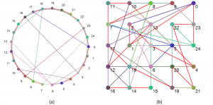
A Boolean network is simply a set of connected nodes. Each node can adopt one of two states: 0 or 1 (hence ‘Boolean’), and has associated with it a rule that relates the next state of the node from the current states of the nodes that are connected to that node. Connections in Boolean networks have direction. If A is connected to B this means that information can flow directly from A to B. It does not follow that information can flow directly from B to A, unless B is also connected to A. This does not exclude the possibility that B is part of a feedback loop that eventually feeds-back to A. Figures 1a and 1b show pictorially the Boolean network that is used throughout this study. The two figures represent the same network, just drawn differently.
Boolean?‘Small?World’?network?used?for?this?study
The red connections indicate that the nodes are connected in both directions
Figure 1 just illustrates the network’s static topology. Figure 2 shows the same network in tabular form, but also includes the all-important Boolean rule that is associated with each node, and which is used to process/transform the information (the collection of states) from incoming connections. We can see here that the number of incoming connections to any one node ranges from 1 (Nodes 6, 7, and 14) to 5 (Node 12).
The?Boolean?rule?and?set?of?incoming?connections?from?other?nodes?for?each?node?in?the?network
To understand how the Rule determines a node’s next state, let’s consider node 10, which has two inputs (or neighbors–nodes 8 and 11), whose states are combined via the Rule 0xB (hex for 1011 in binary). Table 1 shows how different combinations of the node 10’s inputs are processed:
Table?1
Rule table for Node 10. Note that the rows of the third column combined are 1011, or 0xB. This is the Boolean rule for Node 10.
| Node 8 state | Node 11 state | Resulting Node 10 State |
|---|---|---|
| 0 | 0 | 1 |
| 0 | 1 | 0 |
| 1 | 0 | 1 |
| 1 | 1 | 1 |
Network structure
Before looking at the dynamics of this network in detail there are number of measurements we can extract to characterize the network’s static topology. Table 2 lists a number of important metrics that characterize this network.
Table?2
Topological metrics for the network of interest
Most of these metrics will be very familiar to those studying networks. At the simplest level we have a network containing 25 nodes and 75 connections between those nodes. The network has an average outdegree (outgoing connections) of 3 and an average indegree (incoming connections) of 3. We can also see that this network can be best described as a ‘Small World’ as the average path length (the average of the shortest distance between any two nodes) is only 3.55–compared with a diameter (shortest distance between two most distant nodes) of 8. The number we’d like to highlight is the number of structural feedback loops: 2345–a surprisingly high number perhaps to those not familiar with the challenges of understanding network dynamics. Even relatively simple networks, such as this, can have support very complex dynamic behavior.
Most readers will be familiar with the three-body problem in classical mechanics (https://en.wikipedia.org/wiki/Three-body_problem). Essentially, the nonlinear mathematics for a gravitational system containing only two bodies is relatively trivial; it is analytically solvable. Adding just one more body, therefore creating a three-body system, changes all this and all of the sudden the mathematics is far from trivial and the system’s dynamics becomes chaotic (in the formal mathematical sense). As you’d expect, the problem is rapidly exacerbated as more bodies are added to the system. In short, the three-body problem is an example of the challenges of predicting the ‘paths’ of systems containing more than two nonlinearly connected bodies/nodes. The challenge of prediction for chaotic systems is well-known.
The reason we bring this up is simply to illustrate the challenge of understanding the dynamics of even simple networks. The three-body problem can be represented as a 3-Node network containing only 4 feedback loops–the network of interest herein has 2345–what chance do we have of understanding this?!
For completeness the full structural feedback profile of the network above can be written as: 20P2, 16P3, 7P4, 4P5, 10P6, 29P7, 40P8, 51P9, 61P10, 75P11, 137P12, 254P13, 366P14, 401P15, 340P16, 243P17, 153P18, 82P19, 38P20, 15P21, 3P22. “20P2” says that there are 20 structural feedback loops with period 2.
As the discussion above suggests, studying the dynamics of even relatively simple networks is an enormous challenge. What we need are tools and methods for somehow reducing the complexity and yielding reliable insights about the whole by studying subsets of that whole. Seems reasonable, until we add into the mix Cilliers's observation that complex systems are themselves irreducible2.
Taken literally, Cilliers’s observation would suggest that there is little we can do to overcome the fundamental limitations of simplifying complexity–bearing in mind that Science itself is really nothing more than constructing and testing simplifications of observable reality, we seem to have reached a point where Science itself cannot proceed. However, it has been shown (e.g., 3) that reliable and robust, and even insightful, simplifications of complex systems can indeed be extracted, as long as we remember that any conclusions drawn from those simplifications must be applied with care.
Returning to our Boolean network, our next step is to explore the dynamics of our network of interest. The Boolean network analyses were conducted using a tool developed by one of the authors over a number of years that runs on Microsoft’s .NET framework.
Figure 2 shows the rules used by each node processes incoming information (other node states). By randomly seeding each node with 1 or 0 at time = 0, the network is simulated forward in time (setting time = time + 1 at each step) by applying the rule for each node as illustrated in Table 1. If the macroscopic network state is taken to simply be the result of concatenating the states for each of the nodes, we can easily visualize the time-dependent behavior of the network. Figure 3 is example of the time-dependent behavior of this network given a random initial condition.
The?state-time?diagram?for?the?network?of?interest
The state-time diagram for the network of interest. Node 0 is the right-most column, with Node 24 being the left-most.
The initial state, the first row of pixels, is shown in red. This is the state of the network at time = 0. Each of the subsequent rows shows the state at the next epoch. So, for example, Node 0 switches from 0 to 1 at time = 2.
Given that the state space of Boolean networks is discrete and limited (225 = 33,554,432 states in the case of a 25 node network) the network will eventually get back to a state it has visited before, and the network’s behavior is said to have reached an attractor on which its behavior will repeat forevermore (unless perturbed externally).
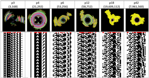
The dynamic (phase) space, as opposed to the topological (structural) space, of any given (Boolean) network is characterized by a number of dynamic cycles, or attractors, i.e., all possible network states can be mapped onto an attractor in phase space. For this particular network we find that there are 2p3, 10p4, 3p6, 3p12, 1p18, 1p42 attractors. This expression is read much the same way as the structural feedback loop expressions given above, e.g., 2p3 represents 2 phase space attractors with period-3.
Figure 4 shows six of the phase space attractors for the network of interest, and their respective state-time diagrams. At the center of each attractor is the attractor basin, and connected to each state in the basin are transient branches that show how the network progresses from any state to eventually ‘fall’ into one of the basins.
The number and type of attractors is a way of visualizing and characterizing the ‘function’ of the network. For example, in biological regulatory networks the genotype is the structural network itself, and the phenotype is the various attractors that ‘emerge’ from the genotype (https://en.wikipedia.org/wiki/Genotype-phenotype_distinction, 4). Alternatively, we have a way here to associated form (structure) with function (dynamics).
The?phase?space?and?state-time?diagrams?for?6?of?the?20?attractors?for?the?network?of?interest
Node 0 is the right-most column, with Node 24 being the left-most.
Table 3 provides a summary of the phase space characteristics of this network. In short, there are 20 quantitatively different attractors, and 6 qualitatively different attractors (i.e., attractors with different periods) with periods ranging from 3 to 42. There is a single 18 period attractor that accounts for 58.4% of all phase space states, and the longest transient, i.e., the largest number of steps between a state not associated with an attractor basin and a state on an attractor basin, is 117.
Table?3
Summary of phase space characteristics of given network
Dynamic structure
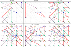
You may have already noticed, from Figure 4, that some of the nodes seem to be fixed in the state-time diagram, i.e., their state does not change at all whilst in certain attractor basins. A fixed state suggests that no information is flowing through that node, or to put it another way, the multiple flows of information around the network conspire to ‘freeze’ some of the nodes. These nodes effectively become ‘walls of constancy’, or information barriers, through which no information flows.
An interesting characteristic of Boolean networks, and perhaps this extends to all complex networks, is that, as far as network function is concerned, any nodes that are frozen/inactive in all attractors can safely be removed without affecting the function of the network3. For some networks (but not the one under study herein) the emergence of frozen nodes can result in the modularization of a network, in which the network is effectively carved-up into independent sub-networks, or components. The point is that for any given attractor not all the nodes contribute, and so there is a sub-structure that is responsible for the observed dynamics that is a subset of the overall network structure–static structure and effective dynamic structure can be very different things.
To illustrate this distinction further Figure 5 shows the effective dynamic structure for each of the attractors (functions) shown in Figure 4.
It is tempting to suggest that the nodes absent from each view contribute little to the network’s dynamical behavior. However, not only is it important to realize that a node that plays a small role in one function, may actually play a very special role in another (and all the possibilities in between), it is also essential to remember the importance of a ‘container’ for emergence to occur within.
In Glenda Eoyang’s Conditions for Self-Organizing in Human Systems5 thesis, she presents her CDE Model (Container/Difference/Exchange), in which the “Container bounds the system of focus and constrains the probability of contact among agents.” The inactive nodes in the network under study represent such a container within which the other nodes can interact and exchange information that contribute to the particular function that emerges. Notably, even though the whole network itself can be seen as a container (the very fact it is a network ‘contains’ the system considerably), the dynamic shape of that container is co-dependent on the attractor (function) being exhibited–the container itself is emergent; a node is ‘frozen’ as a result of the net effect of the 2345 interacting feedback loops.
Ensuring that removal of the frozen nodes left the compressed network functional equivalent to the original network would require checking that the node was frozen in every attractor. Even then, removal of the frozen nodes would still reduce the DR of the compressed network. So, compression needs to be considered in context. As we are analyzing the structural properties of the (dynamically) compressed graph in this paper, we do not have to apply such thorough criteria–fortunately, as checking all the attractors would be computationally intractable using the resources available to this stage of the research.
Effective?dynamic?structures?for?selected?attractors
Shannon entropy as a measure of activity
Another way to partition (and so simplify) the network is to ‘layer’ it by considering the activity of each node. As a metric for activity we’d like a measure that was zero if the node state was ‘frozen’, and close to unity when the node was very active. After some trial and error, we found that the Shannon Entropy (https://en.wikipedia.org/wiki/Entropy_%28information_theory%29) of the state sequence for each node provided the appropriate activity profile–it provides a measure of the information contained in the node activity. The node state sequence is simply the state of a given node as it changes in time. So for a frozen node this might be ‘0,0,0,0,0,0,0,…’; this contains no information, and above is referred to as an information barrier.
The Shannon Entropy, H, of a particular node state sequence is calculated as:
Where P(x) is the proportion of 1s (or 0s) in the state sequence. Figure 6 shows the Shannon Entropy for each node when the network is in one of the attractor basins. The cells have been colored to indicate nodes with high Shannon entropy and those with low; the lowest being the red ‘frozen’ nodes. The table rows have been ordered by each node’s total entropy across all attractors, and the columns have been ordered by the number of red ‘frozen’ nodes in each attractor.
Shannon?Entropy?for?each?node?operating?within?each?attractor?basin
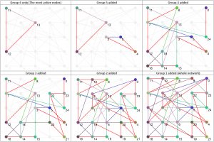
Using the data presented in Table 4 allows us to ‘layer’ the network now in a different way, by grouping the nodes based on their Shannon Entropy, or activity. The group number is given in the last, rightmost, column. Similar to what is shown in Figure 4, Figure 8 provides six different views that, starting with group 6 (Nodes 11, 12 and 13), sequentially adds each group to the network structure until we arrive at the whole original network.
It is somewhat expected that Node 12 (and it's direct neighbors: Nodes 11 and 13) is the most active Node given that it has the largest number of incoming connections. Although, bear in mind that this has as much to do with Node 12's Rule as it is with the number of incoming connections.
Effective?dynamic?layers?based?on?node?Shannon?Entropy?group
Shannon Entropy Signatures (SESs)
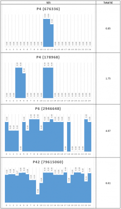
Another way to visualize the dynamic behavior of the network of interest is to construct their Shannon Entropy (SE) profile or signature. For each attractor the SES is simply a column chart showing the SE for each node. Figure 8 shows the SESs for four of the network’s attractors.
Shannon?Entropy?Signatures?for?four?attractors
Again, the dominant nodes in the p4 attractors are readily apparent.
If, via a small external perturbation, the network was pushed from a p4 attractor to a p42 attractor for example, we could say that the network has moved from a modular, low information (0.85) mode to a distributed, high information (6.61) mode. In this way, it might be possible to determine different operational modes in real networks, once a proxy for SE is determined.
Furthermore, rather than developing a set of archetypes for the different ‘connectivity modes’ and ‘information levels’ that the current network behavior might be mapped to, the focus would be on how the SES changes over time. In this way, we can monitor for qualitative changes in the SES, wave a flag to announce such a change, and then consider the significance within the network of interest of such a qualitative SES change. As mentioned in the introduction, some of these ideas are somewhat speculative, but we believe that by using insights from Boolean network analysis, robust general-use network tools can be developed.
Discussion and conclusions
The aim of this paper in some ways is to make the obvious point that a pre-occupation with network structure in the absence of dynamic considerations can lead to very misleading insights into how one might interact with a real-world complex network. In the presentation above it is clear that a purely topological analysis of the original network ‘graph’ would not capture some of the structural properties that only become apparent when dynamical, functional, and phase space analysis is performed.
An alternative way to "slice" the network was also presented based on each node's Shannon Entropy. A Shannon Entropy measure was applied to the networks, allowing them to be layered (from dynamical considerations) to aid visualization, while also providing a way of obtaining an information-based network signature. Further work will be required to see how these approaches can provide real-world insights.