Introduction
Evolutionary computing in various forms has been used previously in complex systems research such as emergent computation1, the dynamics of complex networks2, and also directly in optimal power flow (OPF) research3, while complex systems thinking constructs synergies between the concepts of neo-Darwinian evolutionary processes and the studies of systems and their structures to gain understanding of how the latter may transform in response to their environment4. This work explores a method of addressing the configuration of large-scale electrical power networks, such as a national grid, using an approach based on evolutionary computing to perform multi-objective optimization.
The method used here goes some way to answering questions such as how might a new infrastructure be composed in terms of DG units, how are its components geographically distributed, and how many of each type would be most appropriate given cost constraints.
One of the essential problems in electrical power networks is that of power flow and OPF calculations of alternating current (AC), and these calculations are at the center of Independent System Operator (ISO) power markets5 in which AC OPF is solved over a number of different orders of magnitude of timescales, from minutes via hours, to annually and multi-year horizons, where the latter is for planning and investment while the former are for ensuring demand is met and for spot market pricing. The ISO produces and acquires load forecasts, receives offers of power from generating companies acting within a competitive auction market, and produces generation schedules consisting of required power units and a price, to meet demand within the constraints of the grid and generators.
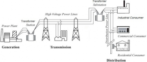
General?large?scale?grid?network
A schematic diagram of a general large scale grid network7.
The power network, for example Figure 1, can be improved both technically and economically through the inclusion of distributed generation (DG) which may include renewable energy sources. DG units are lower output generators that provide incremental capacity at specific geographical locations, thus enhancing voltage support and improving network reliability while also acting economically as a hedge against a high price of centrally produced power, through locational marginal pricing (LMP). LMP creates prices at short intervals, such as five minutes, and causes the price to reflect the value of the energy at the specific location and time it is delivered, in terms of generation cost but also demand, and depends on how congested the transmission system is, since in a congested system the cheaper electricity may not be available in certain locations. The operation of grids by ISOs as unbundled auction wholesale spot power markets that support real-time pricing provides a further incentive to roll-out DG, thus arises the need to define the type, number and location of extra DG units6.
The work presented here addresses the composition of a DG AC electrical power network based upon the IEEE 30 Bus Test Case which represents a portion of the American Electric Power System (in the Midwestern US) in December 1961, and which was downloaded from8. This network, as shown in Figure 2, is amended to have six central fixed large-scale open cycle gas turbine (OCGT) electrical power stations, and twenty four variable distributed generators, powered either by renewable energy sources, being solar photovoltaic (PV) or micro-wind turbine, or by micro gas turbine. In particular, this work uses historical data of weather (in the form of actual solar PV and wind power generation), central power generation, and electrical energy demands, from Australia of 2010, thus providing a realistic simulation environment for both demand and renewable generation.
The aims of this work are two-fold: (a) To determine the composition of the power network in terms of the type, number and location of the non-central DG units, with the goal of finding the cheapest configuration (capital cost), of meeting demand for power while keeping over- and under-production of power as low as possible, and of minimizing the spot price and CO2 emissions, thus determining the best, or at least high performing candidate network solutions; (b) To analyse the multi-dimensional results of the evolutionary computation component in order to reveal relationships between the network's design vector elements, by means of most influential nodes and type of technology, as well as tipping points in the behaviour of the system.
Procedure
Background
The Plexos tool9 is incorporated to provide both OPF and financial market simulations, in particular providing unit commitment (which generators should be used, bearing in mind their operating characteristics such as ramp-up time as well as power output and running costs), economic dispatch (which generators to use to meet demand from a cost viewpoint), transmission analyses (losses, congestion), and spot market operation. It also provides estimations of CO2 emissions. The volume of lost load (VoLL) is the threshold price above which loads prefer to switch off, while the dump energy price is that below which generators prefer to switch off, and these along with market auctions also contribute to the ratio of power generated to power consumed. Transmission losses are also taken into account within Plexos through sequential linear programming.
Plexos is integrated with a multi-objective optimizing evolutionary algorithm (MOOEA)10, thus establishing an optimization feedback loop, since Plexos gives optimal unit commitment for a given set of DG units, while the MOOEA is used to determine the optimal set of generators for the given demand profile and weather pattern. A MOOEA is used as they have a history of tackling non-linear11 multi-objective and multi-dimensional optimization problems successfully, and since OPF for AC power is a non-linear problem while power markets require multi-part non-linear pricing. In the model used here, there are seventy two parameters that constitute the design vector applicable to each candidate solution, represented as one individual in the MOOEA, thus the problem is both non-linear and multi-dimensional. The simulation has a horizon of one calendar year, represented as 365 steps of 1 day increments with a resolution to 30 minutes, from 01-Jan-2010.
A MOOEA12 is generally an heuristic, stochastic means of searching very large non-linear decision or objective spaces in order to attempt to obtain (near) optimal or high-performing solutions13 for problems upon which classical optimization methods do not perform well. EAs are characterized by populations of potential solutions that converge towards local or global optima through evolution by algorithmic selection as inspired by neo-Darwinian14 evolutionary processes. An initial population of random solutions is created and through the evaluation of their fitnesses for selection for reproduction, and by the introduction of variation through mutation and recombination (crossover), the solutions are able to evolve towards the optima.
MOO gives rise to a set of trade-off solution points15 since all objectives are optimised simultaneously, giving rise to individuals that cannot be improved upon in one objective function (OF) dimension without being degraded in another. When each remaining solution in the population cannot be said to be better than any other in all OF dimensions, they are called non-dominated and are members of the local Pareto-optimal set, and are all of equal value and potential interest to the researcher. The non-dominated set of the entire feasible search space is the global Pareto-optimal set12.
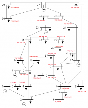
IEEE?30-bus?test?system
The IEEE 30-bus test system in single line diagram style16, showing the location of DG units by bus (node) as numbered in large bold. The V-number is that of the variable holding the number of DG units assigned for the associated DG type at that bus as cross-referenced in Table 1. The circle with tilde indicates a large central generator input and the down arrow indicates bus output to a load.
Method
The evolutionary algorithm used here is a multi-objective optimizing genetic algorithm that self-adapts its control parameters, where the term self-adaptive is used in the sense of Eiben et al.17 following on from the work of Bäck18, to indicate control parameters that are encoded in the internal representation of each candidate solution along with the problem definition parameters applying to the objective functions (the main parameters), and that these control parameters are subject to change along with the main parameters due to mutation and crossover. This is different from a purely adaptive control parameter strategy as in that case the change is instigated algorithmically by some feedback at the higher level of the genetic algorithm (GA) rather than the lower level of each chromosome/solution in the population. The deterministic approach is rule-based and is not considered adaptive.
The Plexos tool is used here as the source of the values of the objective functions that are evaluated and selected for, that is to say, the fitness indicators, by the MOOEA, as depicted in Figure 3.
MOOEA
The integration of Plexos with the self-adaptive multi-objective optimization algorithm.
The problem is defined as a set of potential DG units each of which may or may not be located at a given node (bus). The DG units are defined as (i) micro-gas turbine (ii) Wind turbine and (iii) Solar photovoltaic, where a unit of value 0 means the generator is not present at the location. The scenario allows for up to 5 units of each type to be located at any of the nodes defined as variable in the network diagram (Figure 2), which means that it is any except for the nodes 1, 2, 13, 22, 23 and 27, as these are the large fixed central OCGT power stations.
The labels shown as Vn at the given nodes indicate the design variable number that defines the number of units of the given generator types at that bus, and as can be seen, each of the 3 variable types can be present potentially. As there are 24 nodes at which variable DG units can be located and 3 types of generator, the design vector of each candidate solution therefore consists of 72 variables. A candidate solution is therefore a vector of n decision variables: =(x1,x2,…,xn) , where n = 72. This configuration thus allows a solution to have from 0 DG units up to a theoretical 360 (being 5 units of each of 3 DG types at the 24 nodes). Table 1 below shows the allocation of DG units by type to nodes, cross-referenced to its variable number (as shown in Figure 2), with the assumption that a given generator feeds in to one associated node only.
There are 4 objective functions defined, all of which are to be minimised simultaneously and the values for all of which come from Plexos, these being:
Eq. 1 min F(genCost) = genCost
Eq. 2 min F(useDump) = | useDump |
Eq. 3 min F(spotPrice) = spotPrice
Eq. 4 min F(CO2) = CO2
in which the values represent respectively:
The generation cost (in currency, e.g. $)
The USE/DUMP energy (MWh)
Spot Price ($/MWh)
CO2 emissions (Kg)
Considering the values above, useDump, depending upon whether it is negative or positive, is respectively either the un-served amount of energy due to under-production or the dump energy due to over-production, relative to demand. By minimizing the absolute value of useDump, the optimization seeks to make this value approach zero, that is to say, to try to make the supply match the demand, thus obtaining the most efficient system. The spot price is the mean price achieved in the simulated market auctions over the course of the simulation, in Plexos.
A hard constraint, sumU, on the total number of DG units deployed, u, is applied in Equation 5, in order to investigate how the system transforms itself. Without such a constraint, which can be viewed as a limit to financial resources available as investment into DG, we would perhaps expect the system to maximize DG deployment since they provide a known benefit and where cost is the only downside, and this would hide the effects that placement may have when otherwise.
Eq. 5
The hard constraint is increased in other runs to see what effect a larger number of allowed units may have, as shown in Equation 6:
Eq. 6
The candidate solutions chosen by the MOOEA, using the results from Plexos, are thus selected due to the effect their chosen DG units have on the electrical network due to their operating characteristics and where they feed into the network, defined in the topology as shown in Figure 2.
The MOOEA allows each new experiment, such as the one defined here, to override its default initializer which creates an initial population of candidate solutions by generating variables under a uniform random distribution regime within the ranges of the defined variables, in this case 0 <= u <= 5. The initializer used instead generates solutions that meet the hard constraint, by selecting for each solution a random value between 0 and the constraint, 70, and using this as the limit for that candidate solution. Each variable of that solution is then selected randomly, and is allocated a random value within its range, until the solution's own limit is reached. In this way, solutions in the initial population will vary between 0 DG units and 70 with a uniform distribution.
In subsequent generations, solutions will evolve that may break the hard constraint, due to mutation and recombination operators acting on ‘fit’ parent solutions selected for breeding, and in this case the solutions will be retained in the population but repaired. Repairing in this context means that a failing solution's vector of DG variables is changed until it falls within the constraint, by randomly choosing one of the variables, decrementing its DG unit count (when it has u=1), and then repeating the process until the total falls within the constraint.
The MOOEA is configured to have a mixed chromosome consisting of a vector (the genes) of 72 integers, with the self-adaptive control parameters encoded as real numbers. It has a fixed population of size 30, allows 0 duplicate solutions in any given generation, has initial crossover and mutation probabilities of 0.9 and 0.01389 (= 1/72) respectively and is allowed to run until all solutions are non-dominated or until 5 days have elapsed, whichever is sooner (since each generation takes in the region of 3 to 4 hours elapsed time, which increases as the generations increase, apparently).
Table?1
The nodes, their generators and generator types.
Results
The results are given as 2D scatter plots and higher dimensional plots using the parallel coordinates (?-coords) technique19,20,21,22, in which each dimension is oriented parallel to the others, thus transforming an n-D point into a polygonal line. The latter technique enables multivariate data to be plotted uniquely and without loss of information, and in these cases the whole design space of each solution, 72 variables, are plotted alongside their objective function results, and also with the sum of the DG units assigned (sumU) as in Equation 5.
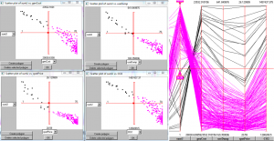
Scatter?plots?of?four?OFs
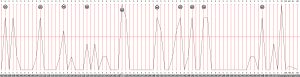
Scatter plots showing sumU on y-axis and (a) Top left: genCost (b) Top right: useDump (c) Bottom left: spotPrice (d) Bottom right: CO2, and on the right a ?-coords plot showing a selected region of higher sumU which corresponds to lower OF values. Hard constraint on sumU = 70.
Figure 4 concerns results obtained when the hard constraint of 70 was applied to sumU, and the scatter plots of show the sumU plotted against the four OFs as described in Equation 1 through Equation 4, from which it can be seen that there is broadly a trade-off between the number of DG units deployed and the quality of each of the other OF values. An obvious optimal trade-off front has not yet developed in the course of the optimisation, but the trend is clear, and that is that increasing the number of DG units deployed improves (decreases) the other OF values. The ?-coords plot to the right of the scatter plots emphasises this point, in that there is a narrow region between sumU and genCost in which the lines from sumU cross, itself an indication of anti-correlation, while the lines from genCost to the other OFs to its right are mostly positively correlated. It can be seen however that not all of the lower genCost points lead to the lower useDump points, and indication that possibly a little more central generation was needed under certain circumstances, meaning that supply and demand was not always so well matched.
Also in Figure 4 in the ?-coords plot there is an indication that the system may have a tipping point (bifurcation) dependent upon the value of sumU at around 34 units, as the selected region shown by the two arrows has an upper boundary of 34, and the OFs relating to all these lines seems to be in the top half of the worst performers.
The plots of Figure 6 and Figure 7 also related to the hard constraint of 70 units, and show the best performing solution found for the genCost objective. The latter figure makes it clear that it is the wind turbine DG units (indicated by W) that are the primary contributor to the performance of the best solution for genCost, with variable V32 having the most units allocated, and V11 being the most connected in the network (feeding into node n06).
Hard?constraint?of?200
Shows results when the hard constraint sumU is increased to 200, with scatter and ?-coords plots similar to Figure 4.
The results of Figure 5 are presented similarly to those of Figure 4, but for the hard constraint of 200. The ?-coord plot shows the relationship between the number of DG units and best performing OFs more clearly (when in colour), in that the more DG units allocated, the better the OF performance. Clearly, without the constraint the system would attempt to allocate as many DG units as possible, so the constraint acts as a limit on the cost of DG deployment. The scatter plots of sumU against the OFs also show the clear trade-off trend.
Conclusion
It has been shown that this methodology can indicate not only the number of DG units, but also their type and their network location, in order to gain high performance when used with an appropriate OPF tool such as Plexos. Conversely, this approach could also be used to assist in the design of network topologies, working within the limitations of geography and socio-economic factors, by considering the connectedness of the network either by transmission line connection or by line capacity. For this network and the weather seen in the stated time period, it appears that wind-turbines may be the most important DG technology to deploy, although the other types are important too since all wind DG would be unlikely to equal the performance seen, due not least to its intermittency.
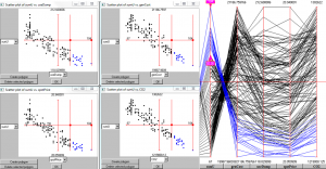
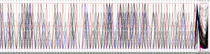
||-coords?plot?of?the?entire?data?set
For HC=70, showing the 72 variables, the derived sumU followed by the 4 objective functions. The best performing point of genCost is shown selected by the two arrows at the far right bottom, and its associated variables shown in blue when in colour. See Figure 7 for a clearer picture.
||-coords?plot?of?the?entire?data?set
For HC=70, showing the 72 variables, the derived sumU followed by the 4 objective functions. The best performing point of genCost and its associated variables are shown, with the rest filtered out. The (W) annotation against a variable indicates that it is a Wind DG unit.