Introduction
In the previous issue, ECO’s classic paper and my introduction to was Robert May’s pioneering work in chaos theory, in particular an exploration of the by now iconic logistic map and its display of a period-doubling route to the onset of chaos. In one of those odd coincidences not infrequently found during the course of scientific discovery, researchers working independently can happen upon similar or even the same findings without knowledge of the others’ work. Such was the case with May and another physicist Mitchell Feigenbaum who was then working at the Los Alamos National Laboratory (an unexpected breeding ground for many chaos and complexity scientists) and had been conducting his own research also into the logistic map. This coincidence edges on the downright eerie when the two papers are placed side-by-side which reveals nearly identical graphs, diagrams, and numerical lists.
These two physicists had ventured into the world of pure mathematics where it was unclear at the start whether their research would yield anything of interest to physics per se. At that time the newly discovered finding of technical chaos was proving significant in several areas of physics due in large measure to the apparent indistinguishability of chaos from randomness, e.g., in turbulence, phase transitions and related critical phenomena. For instance, Ruelle and Takens1,2 had applied chaos-producing functions (coining the expression “strange attractors” along the way) to study fluid turbulence. Indeed, near the end of his classic paper, Feigenbaum himself offers some remarks linking the constantly increasing number of period doublings leading up to the inception of chaos to previous theories of turbulence such as Landau’s which had focused on quasi-periodicity and not chaos (which had not yet been discovered). For the most part, though, interest in the logistic map was taking up mostly in the study of population and other ecological dynamics as in the burgeoning mathematical arena of dynamical systems theory.
Because of the nearness of Feigenbaum’s explorations to those of May, my introduction to May’s article and the article itself are quite relevant to this introduction to Feigenbaum’s classic paper. It is not the case, however, that Feigenbaum’s investigations merely start where May’s left off. Rather, Feigenbaum discovered the totally unexpected presence of two new mathematical constants on the way to chaos, the finding of a constant(s) being a very rare feat in the history of mathematics and one which has no doubt granted Feigenbaum not a small measure of mathematical immortality.
Mathematical constants come few and far between. Perhaps the most well-known being ? (pi), whose discovery is usually attributed to Archimedes although something quite like it was known to other traditions in ancient India, China, … who knows? The most common place where ? is found has to do with metrics defining circles, e.g., as the ratio of the circumference to the diameter of a circle, ?=C/d, or the area of a circle, A=?r2 (radius). It is a constant since its value is invariant with respect to the size or scale of the circle, i.e., a circle whose diameter is double the diameter of another circle, will have a circumference double that of the first, thereby maintaining the ratio C/d, i.e., ?. Since ? is an irrational number, its value can only be approximated as 3.14159… (this is random—as of the year 2000, the value of ? had been computed to 1017 places). Its invariance to scale is just one aspect constituting what’s called the universality of ? as a constant. Even more remarkable is how ? shows up in areas of math seemingly unrelated to that of circles, for example: the probability of two randomly chosen integers being coprime; the probability that a pin dropped on a set of parallel lines intersects a line; anywhere that Fourier transforms are used; the precise sum of the infinite series constituted by the reciprocals of the squares of the natural numbers; all of which would presumably have little or nothing to do with circles3,4. One of the most dramatic displays of ? in mathematics has to be Euler’s identity,
This identity is celebrated by mathematicians because it contains the five most important constants, namely, ?, e, i, 1, and 0 (that latter two numbers 1 and 0 are typically taken as constants for certain mathematical reasons).
Looking at another near ubiquitous constant e should suffice to appreciate what a great accomplishment Feigenbaum has wrought with the discovery of his two. The use of the letter e is usually attributed to either exponential growth or Euler who found great use of it in his awesome mathematical research:
Constants can be interpreted as fundamental universal constraints on what is possible not only mathematically but in relation to the phenomena that the mathematics can be said to represent or model. Thus, ? in regard to circles is invariant in that any circle no matter what size must obey the formula that the ratio of its circumference to its diameter will be 3.14159… If not, then the object is not a circle. In this sense ? helps define a circle as a circle. In other words, it constrains reality to the case (that is, operates as a law of nature) that a round planar figure whose boundary (the circumference) consists of points equidistant from a fixed point (the center) is a circle displaying, these equidistant points making up the circumference which then divided by the diameter equals ?.
Feigenbaum’s constants
Feigenbaum’s discovery of his two new constants opened up an exciting new perspective on dynamical systems, particularly those showing some sequence of bifurcation, period doubling and the onset of chaos. Rather than holding to the antecedent viewpoint which relegated chaos to connotations of unpredictability, instability, and unruly randomness, we know now that these properties are only partial and incomplete. Instead, chaos in its technical sense has its own “built-in” constraints ordering what can happen dynamically and naturally. It’s not that somehow nature arranges things to first be unruly and then clamps down on natural spontaneous activity with boundaries and containment fields. Instead, right from the start, natural processes exhibiting chaos or are on their way to chaos are simultaneously diverging (e.g., shown by Lyapounov exponents) and being constrained to exhibit order and organization. For that is what constants serve to do: they are recognition of constraints, what the ancient Greeks called forms, operating on and through the very substance, the Greek hyle, of things.
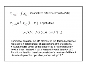
In the classic paper reprinted here, Feigenbaum explores and explains the constants he uncovered by focusing on the relationship between the parameter values of the logistic map and the role of functional iteration, an expression Feigenbaum coined for how the function of the logistic map is continually repeated with each newly arrived-at value of the variable (such as P for population year to year). That is, the new value is pumped back into the formula in an updating fashion. Remarkably enough, Feigenbaum had conducted his research through the use only of a hand-held calculator and not any of the mainframes otherwise presumably engaged in doing calculations on the yield of thermonuclear warheads (his place of employment after all was the Los Alamos National Laboratories; see Gleick’s engagingly written, thorough and prescient new edition of his Chaos: the Making of a New Science—indeed rereading Gleick after close to thirty years has been a very rewarding experience in several ways, one of which is the revealing of those trends in complexity science back then which either went on to make an enduring contribution or have since expired). By the way, over the years since his discovery Feigenbaum has received well deserved awards and faculty positions at prestigious universities, certainly none more prestigious that his current professorship at Rockefeller University.
As a statistical physics, Feigenbaum’s initial motivation appears to have had something to do with taming the unpredictability associated with various manifestation of randomness. Inspired by talks given by such famous dynamists of the time like Steve Smale (see Smale, 5,6 probably the crucial role of iteration in Smale’s famous horseshoe map, and David Ruelle, 1971, presumably his work on using chaos and its strange attractors as models for turbulence). Along the way, Feigenbaum became very intrigued by the whole notion of functional iteration:
Functional?iteration
Although difference equations, e.g., ones with lagged time variables, and their iteration had been in use in various scientific fields such (as the logistic map used in population dynamics), it was May and Feigenbaum who took a special interest in them from the viewpoints of two physicists exceptionally proficient in pure mathematical investigations.
Today is a different story, however, since partly due to May’s and Feigenbaum’s seminal research, functional iteration has become a mainstay of chaos theory and complexity science. This can be seen, for example, in John Holland’s model of Constrained Generating Procedures from his work on cellular automata as a prototype of computational emergence (Holland contending his mathematical formulation could offer a theoretical foundation for emergence in general):
fc: Ic x Sc ? Sc (where fc is defined so that: fc(t+1) = fc(Ic(t),Sc(t)); I = possible input combinations at time t ; S = states of system at time t).
In Holland’s model, transition functions act on input combinations to generate components mechanisms, the function iterated in a similar way to Feigenbaum’s theme of functional iteration. Another example of an explicatory strategy relying on functional iteration but in the completely different field of semantical paradoxes in logic is that of the use of difference equations and their functional iteration representing the deliberations over time of the truth or falsity of self-referential propositions which have been suitably infinitized through fuzzy logic valuations (see an exposition and interpretation of these kinds of models in Goldstein7).
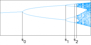
Even with his insights into functional iteration, what Feigenbaum had accomplished so far was little more than what May had already done. Things began to heat up though when Feigenbaum noticed that as the periods increased (such as period 2 bifurcating into a period 4 attractor, period 4 bifurcating into period 8, and so on), the values of the bifurcation parameter became closer to each other as shown in the famous bifurcation diagram in Figure 2 below8.
Feigenbaum next measured the rate at which the bifurcations become closer, which is the rate at which the values of the bifurcation parameter converge to the limit represented by his delta constant: 4.669206…. or, in other words, each new period doubling attractor emergence occurs 4.6669… faster than the previous one:
Feigenbaum’s?Delta?Constant
The horizontal axis is composed of the increasing values of the bifurcation parameter (derived from the birth and death rate plus various ecological resources, threats, etc.). In Figure 3 the points “S” indexed by the counting numbers signify the value of the parameter when period doubling takes place, i.e., the emergence of a new attractor—S0, S1, S2,… , indicate the parameter values where successive period-doubling bifurcations take place:
S0 is the parameter value where the first fixed point attractor becomes unstable and a new, stable period 2 attractor emerges;
S1 is the parameter value where this period 2 attractor becomes unstable and a new, stable period 4 attractor emerges;
S2 is the parameter value where this period 4 attractor becomes unstable and a new, stable period 8 attractor emerges;
. . .
One can see that the distance between S0 and S1 is longer than between S1 and S2—Feigenbaum’s discovery was that the ratio of the successive values of the bifurcation parameter approach a limit (notated as the delta constant below):
Here an are discrete values of the bifurcation parameter at each nth period doubling. Again, the constant shows up as the ratio of the intervals between the bifurcation points as n approaches infinity.
The complexity scientist Melanie Mitchell8 in her highly informative and clearly written survey of complexity science points out another coincidence even closer than that between May’s and Feigenbaum’s research: the team of the french Pierre Coullet and Charles Tresser used renormalization to study period doubling and found the same constant. Mitchell suggests that Feigenbaum may indeed have been first but nevertheless it is often called the Feigenbaum Coullet-Tresser theory and the constant also called with the addition of the French names. This reminds me not only of the infamous controversy over the provenance of the calculus, Newton or Leibniz?, as well as the issue of the justifiable name of the so-called Higgs particle and the Nobel for theorzing about it since about 7 researchers were involved with the first theoretical insights into the role of this “particle” and/or “field”.
Feigenbaum recounts his discovery of another related constant which is customarily overshadowed by the delta constant probably because it seems to drop out, so to speak, from the first constant displayed in the bifurcation diagram of Figure 2. This constant alpha is approximated as a = 2.5029078.., and can be indirectly observed in Figure 2 where the plotting of bifurcation parameter values in the bifurcation diagram displays a figurative horizontally directed tree and branches, or tines and subtines. The alpha constant has to do with the ratio between the width (vertical) of a tine and the width of one of its two subtines (except the tine closest to the fold) (see 11). It is important to note that the bifurcation diagram and the second constant point to a self-similarity among different scales (hence the finding of these constants in various metrics of the Mandelbrot set). This scaling theme became a major aspect of the ramifications of the constants developed by Feigenbaum, a theme that became another cornerstone of complexity studies.
As unexpected as Feigenbaum's discovery of these constaints was, they had a property that was even more astounding, namely, their universality. For instance, it was discovered that the same delta constant value of 4.699...appeared in any dynamical system that approaches chaotic behavior via the period-doubling route to chaos. The delta constant also shows-up in yet more unrelated places (mimicking ? in this eclectic applicability) such as the trigometric sine map, fluid-flow turbulence, electronic oscillators, lasers, chemical reactions and the Mandelbrot set (the "budding" of the Mandelbrot set along the negative real axis occurs at intervals determined by Feigenbaum's constant9).
As long as a function is uni-modal, i.e., has "one hump" when graphically represented, and has a period-doubling route to chaos, the delta constant will be there. A crucial implication of this universality is that the micro-level constituent level (which will differ according to which specific function function is being examined) is not of primary importance in determining the significant dynamical behavior since the constant implies an insensitivity to initial conditions which is just about the opposite of the sensitivity to initial conditions found in chaotic systems (the butterfly effect).
In explaining his finding of universality that goes along with his constants Feigenbaum pointed to the fact that in functional iteration the function is applied to itself recursively so that the iterative operation takes precedence over whatever particular one-hump function is involved: "A monotone f, one that always increases, always has simple behaviors, whether or not the behaviors are easy to compute. A linear f is always monotone. The f's we care about always foldover and are strongly nonlinear. This folding nonlinearity gives rise to universality. Just as linearity in any system implies a definite model of solution, folding nonlinearity in any system also implies a definite method of solution" (p. 21: this definite method would henceforth include his constant and its accompanying mathematical accouterments).
Conclusion
Feigenbaum recognized that scaling was one of the keys in his discovery of universality in a kindred fashion to the place of scaling in the method of renormalization which was then being applied to phase transitions and related phenomena as well as in quantum field theories (see 10,11). In more recent times, universality via scaling and renormalization has become a major tenet of theorizing about emergent phenomena in solid state or condensed matter physics. For instance, the Nobel Laureate Robert Laughlin working with the esteemed physicist David Pines 12 have given the term “quantum protectorates” to such emergent phenomena as superconductivity, ferro-magnetism and the fractional Quantum Hall Effects (Laughlin’s Nobel Prize was for his research in the latter) “characterized by a type of universality that “protects” them micro-level dynamics.
Universality supplies critical insight into understanding lower level or micro behavior since if it is known that universality such as Feigenbaum’s constants are at work, then one can work downwards, so to speak, in order to learn more about the lower level than the usual reductionist explanatory strategy of working upwards from supposed fundamental entities and dynamics. This new strategy promulgated by Laughlin, Pines, and Philip Anderson (another Nobel Laureate for his research into related emergent phenomena) reminds me of the notion of “delving downwards” put forward by the complexity-oriented theoretical biologist C.H. Waddington (see 12 for my introduction to one of Waddington’s classic papers reprinted from and earlier issue of E:CO). An example of delving downwards is how classical laws of organic chemistry as well as classical descriptions of chemical elements and small molecules did not, according to Waddington, sufficiently account for changes in the overall shape of protein molecules containing thousands of atoms. However, when a more global change of shape was discovered, then knowledge could be obtained about the properties of atoms as they were exhibited in molecular groupings.
The higher level “organizing principles” suggested by Laughlin et al. as well as Waddington, need to include the kinds of universal constants discovered by Feigenbaum and others since they act to constrain and thus shape and form lower level micro-constituents. From my perspective we have only begun to uncover the very tiniest tip of the huge iceberg of constants functioning to constrain, channel, bound, limit, shape and form the complex phenomena of complex systems. The world of “big data” which all the hype that has descended upon us must also contain innumerable still unknown constants. The unique and peculiar way that Feigenbaum discovered his constants, though, should provide a guiding principle for unearthing these constants. As he wrote, he would not have come across his constants had he been using one of the mainframe super-duper computers at Los Alamos since he would have simply glossed over and not paid enough attention to the nascent patterns revealed by his numerical simulations on his calculator.
Of course, ever more powerful computers will uncover patterns that unaided human capacities cannot see. But human creativity will still be required in finding what has heretofore been unrecognized. This brings to mind the controversial issue of the new computer driven proof checkers and how innovative proofs are actually discovered. A perusal of several recent autobiographies of eminent mathematicians (e.g., to name two, those by Cedric Villani and Michael Harris) demonstrate that human creativity flows in strange directions with unpredictable twists and turns, leaps of insight, depressing downturns and even reversals and many restarts. We hear about and learn about the great new proofs only after the fact with the unfortunate neglect of the actual creative processes used to get to these proofs.
The original article, published as Fiegenbaum, M.J. (1980). "Universal behavior in nonlinear systems," Los Alamos Science, Summer: 4-27, is available from here.