Stability in the American Automobile Industry:
Insights from Alternate Representations
Daniel Svyantek
University of Akron, USA
Linda Brown
University of Akron, USA
Introduction
The prediction of social system behavior has been traditionally done with research methods based on linear statistical methods. However, many aspects of social behavior may be better modeled using concepts derived from nonlinear approaches to system behavior (Ayers, 1997). The choice between these models is one between alternate representations or means of looking at the world. The statistical approach associated with more traditional systems theory assumes that a few variables, interacting weakly with each other, determine the behavior of systems (Liebovitch, 1998). Nonlinear systems theory, however, proposes that the behavior of systems in the world is affected by many variables that interact strongly with each other.
The remainder of this article will discuss the differences between traditional and nonlinear research representations and their implications for the study of system behavior; provide an introduction to the concept of the attractor and describe a common representation used to analyze nonlinear systems, the phase space diagram; provide an illustration of the use of the phase space diagram to understand stability and change in the US automobile industry; and discuss the results found in terms of the complex adaptive system and organizational culture literature.
TRADITIONAL AND NONLINEAR RESEARCH REPRESENTATIONS
Traditional and nonlinear research methods differ in how experimental data is gathered, analyzed, and represented (Svyantek & Brown, 2000a, 2000b). Traditional research methods use linear methods (e.g., regression) in which independent predictor variables are used to make predictions about a system behavior (the dependent variable). The data gathered tend to consist of (a) individual measures of the predictor variables gathered at Timex; and (b) individual measures of the system behavior gathered at some later time, Timex+1. The predictions made by traditional research methods are quantitative. The value of these predictions is based on (a) the statistical significance of the relationship between the predictor and dependent variables; and (b) the variance in the dependent variable accounted for by the predictor variables. The results of such an experiment are then used to draw inferences about behavior at a future time or in a different context. The forms of data representation used with traditional research methods tend to depict numbers (e.g., a bar graph) or distributions of variables (e.g., a confidence interval).
Nonlinear research methods, however, utilize a different approach to the analysis of data. The data gathered consist of multiple measurements of both independent and dependent variables. The relationships between data are then graphed across some interval of time. The predictions made with nonlinear research methods are qualitative. The value of these predictions is based on the degree to which a consistent pattern of behavior is found in the system across the repeated measurements. The representation forms include simple graphs and more complex descriptions of system behavior known as phase maps. The graphed results of such an experiment are used to make predictions about a system that are more context specific but also more cognizant of the patterns of change in system behavior across time.
The difference between problem representations used in traditional and nonlinear research methods parallels a distinction made in the area of statistical graphics. Graphics have traditionally been used to communicate and store information in scientific works (Wainer & Velleman, 2001). Traditional graphing representations depict numbers or distributions, which are the types of information provided by the graphic representations used in traditional research methods (e.g., the bar graph or confidence interval). New statistical graphing techniques have been developed to depict relationships among variables (Wainer & Velleman, 2001). The problem representations used in nonlinear research methods are well suited to this new interest and may be used to depict relationships among variables.
Nonlinear research methods and concepts have been shown to have heuristic, explanatory value for understanding social systems. An important theoretical concept is the attractor. The nonlinear research technique used to examine attractors is the phase space (Svyantek, 1997; Svyantek & DeShon, 1993; Svyantek & Snell, 1999). The next section introduces these two related ideas.
ATTRACTORS AND PHASE SPACES
One of the seeming contradictions of the study of nonlinear system behavior is that prediction of a nonlinear system behavior is possible from seemingly random behaviors of the system gathered across time (Gleick, 1987). Behavior that at first appears inconsistent or random at one level of analysis becomes predictable as more data are gathered and graphed. The interpretation of the graphs, however, is made at a higher level of analysis. Therefore, multiple measurements of the system behavior must be gathered across time to define this pattern of nonlinear system behavior. The importance of the graphical representation form is that it provides the investigator with a picture of the relationship between variables across time.
Attractors represent a qualitative prediction of behavior of a complex system across time. They represent stable boundaries for the behavior of the system (Hastings et al., 1993). The attractor represents a feasible set of alternatives for system behavior from Timei to Timei+1. Future system behavior will remain on this attractor in the phase space. As the system changes from Timei to Timei+1, the location on the attractor from Timei to Timei+1 is not predictable, but system behavior will remain on the attractor. Therefore, prediction is possible at this higher level of analysis, the attractor, for nonlinear system behaviors.
Nonlinear systems theory provides several means of developing a “geometry of behavior” that can be used to describe nonlinear system behavior and change (Kellert, 1993). An important means for representing the patterns of nonlinear systems is the phase space diagram. Phase space diagrams have been used in the description of different phenomena relevant to the study of organizations, including ecosystems (Hastings et al., 1993); the stock market (Savit, 1991); customer complaints in a governmental agency (Kiel, 1996); the relationship between investment in technology and return on investment in the semiconductor industry (Hutcheson & Hutcheson, 1996); and the evaluation of the effects of organizational change interventions.
A phase space diagram is a map representing the dynamic behavior of a system (Briggs & Peat, 1989) and illustrates the way in which a system transforms itself across time. Phase spaces allow the qualitative evaluation of nonlinear systems by defining those systems' attractors (Kiel, 1996). The attractor defined within the phase space is a pattern or representation of the flow of behavior with a system across time. The phase space diagram may be used to define system attractors (Briggs & Peat, 1989); show the temporal evolution of a nonlinear system's behavior (Kiel, 1996); and provide temporal information on the development of radically new system behavior (this would be defined by a radical change in the location of the system behavior in the phase space diagram) to guide the search for environmental variables that cause these changes (Briggs & Peat, 1989; Kiel, 1996). One analysis of nonlinear systems' behaviors, therefore, starts with the examination of the attractors formed in phase space diagrams (Kiel, 1996).
The analysis of data in a phase space diagram requires repeated measurements of a system behavior across time to understand patterns of variability in the individual data being used to assess macro-level behavior (Abraham, Abraham, & Shaw, 1990). The most simple phase space is the lag phase space diagram. Here, the investigator is interested in change in one variable across time (Liebovitch, 1998). The lag space diagram is created by mapping the change in the variable of interest, y, between Timex-1 and Timex.
The temporal evolution of the system, therefore, is of interest to the investigator when a lag phase space diagram is created. This variable provides information on whether or not system behavior varies across time and the degree to which this variation occurs at particular periods of time or across the entire time period being examined.
The creation of this phase space is relatively simple for many organizational variables of interest (Kiel, 1996). First, multiple measurements of the variable being examined must be gathered by the researcher. One problem with the study of organizationally relevant, nonlinear system behaviors is that there is no clear agreement on how many multiple measurements are required. The estimates of repeated measures required to define an attractor range from 10 to 5,000,000,000 (Liebovitch, 1998). Most data sets available consist, at best, of a few dozen data points across time; this number has been shown to be adequate for tracing organizational attractors (Kiel, 1996; Svyantek & Snell, 1999). These multiple measurements represent repeated measures across time, not subjects, for the variable of interest.
Secondly, the researcher must create a lag variable. This can be done using standard statistical packages such as SPSS (see Svyantek & Snell, 1999, for a complete description of a step-by-step procedure for creating the lag phase space diagram). The lag variable, a researcher-created variable, represents the Timex-1 measurement for each Timex measurement. For example, if the system behavior at Timex-1 is 9 and at Timex the system behavior is 8, the coordinates for the change from Timex-1 to Timex are (9, 8).
Thirdly, the lagged sets of coordinates created for each time the variable of interest is measured are plotted onto a two-dimensional scatterplot diagram. The variable of interest is plotted on the x-axis of the scatterplot and the lag variable on the y-axis. Finally, the figure formed on this graph is examined to see if it provides a consistent picture of system behavior. If a consistent picture is found, it may be interpreted as supporting the conclusion that an attractor exists.
QUESTION EXAMINED
This study used lag phase space diagrams to investigate patterns of outcome behavior for the corporations that make up the US automobile industry. It looked at the market share percentages of the companies comprising the industry during a 27-year period from 1965 to 1992. The companies investigated were American Motors, Chrysler, Ford, and General Motors. The market share value was defined as the number of cars produced in the US that were sold during a month. The monthly market share values were taken from Ward's Automotive Yearbook for each company during this time period. This provided 324 data points (27 years times 12 months) for each company (except for American Motors, which went out of business in 1987). Lag variables were created using SPSS for each of the four companies' market share values. The phase space diagrams were then created based on the 324 data point pairs for each company using SPSS. Market share value is graphed on the y-axis; market share lag value on the x-axis. The scales for the x- and y-axes for each company were made the same to render visual comparisons easier.
Table 1 lists the descriptive statistics for the four US automobile manufacturers studied here. It gives the mean market share and standard deviation values for each of the four companies across the 27-year period.
| Company | 1965-1969 | 1970-1974 | 1975-1979 | 1980-1984 | 1985-1989 | 1990-1992 |
|---|---|---|---|---|---|---|
| American Motors | 3.21 (0.46) | 3.73 (0.81) | 2.69 (1.13) | 2.36 (0.52) | 1.20 (0.37) | ****** |
| Chrysler | 17.16 (1.42) | 16.75 (2.45) | 13.26 (1.87) | 11.74 (1.36) | 13.77 (1.05) | 10.66 (1.53) |
| Ford | 26.86 (3.31) | 29.13 (3.83) | 27.17 (1.86) | 23.38 (2.24) | 27.56 (2.44) | 26.83 (1.46) |
| General Motors | 52.73 (2.72) | 50.40 (6.08) | 56.45 (2.45) | 60.37 (2.72) | 51.13 (4.43) | 44.81 (2.28) |
| Total Big 4 | 99.96 | 99.99 | 99.57 | 93.82 | 93.66 | 82.3 |
Table 1 Market shares for US automobile industry, 1965-92
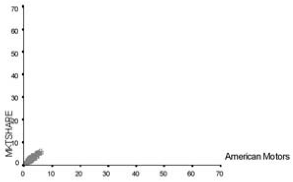
Figure 1 Phase space for American Motors 1967-92
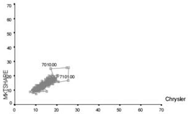
Figure 2 Phase space for Chrysler, 1967-92
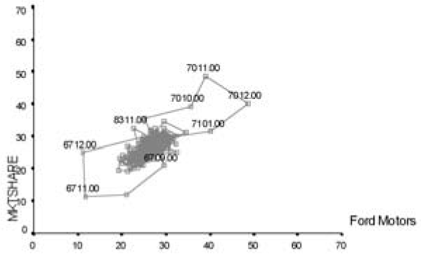
Figure 3 Phase space for Ford, 1967-92
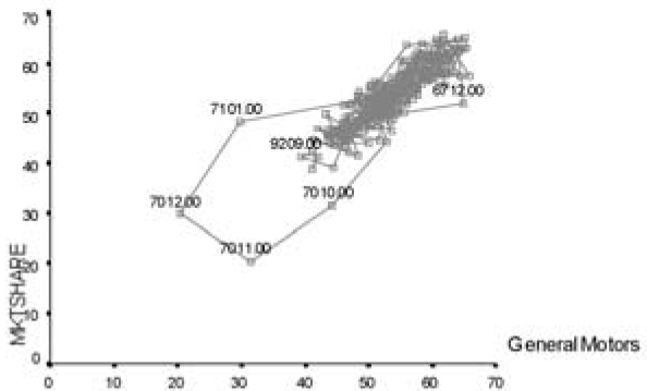
Figure 4 Phase space for General Motors, 1967-92
Figures 1, 2, 3, and 4 are the lag phase space diagrams for American Motors, Chrysler, Ford, and General Motors, respectively. Each graphs the respective company's market share and market share lag variable across the time period.
The phase space diagrams were assessed to see if they provide the information to suggest whether attractors exist within the US automobile industry. Inspection of the diagrams provides support for the proposal that, for market share, attractors may apply for the US automobile industry.
First, each of the four lag phase space diagrams shows an attractor region for the variable, market share, for each of the four companies. This area is consistent across for each of the four companies across the 27-year period of this study. These regions may be interpreted as the characteristic performance level for each company in the US automobile industry.
Secondly, the phase space diagrams also provide a means for understanding the temporal evolution of the attractor region. This may be seen in the change in the fluctuation of market share. Here the figures show an interesting phenomenon. This region becomes more constrained across time. Variation (here defined as the change from Timex to Timex+1) is most pronounced in earlier years of the data studied (1967-71). Each company's attractor for market share, however, becomes more constrained across time and variation decreases.
Thirdly, the phase space diagrams do not provide any support (based on market share outcomes) for the idea that there has been the creation of radically new system behavior affecting the competitive position of the four companies during this period. The relative rankings in terms of market share for the four companies studied remain constant across time. No company develops a competitive advantage that allows it to change its relative position vis-à-vis the other three companies.
Finally, the variation in the figures provides information on when the four companies' market share was most disturbed by environmental events and the direction of this disturbance. Figures 2, 3, and 4 all show the most variation in the early 1970s. The points labeled 7010 (October, 1970) and 7101 (January, 1971) in Figure 3 show the degree and direction of variation for Chrysler's performance on the market share variable. Similarly, the sets of points labeled 6711 (November, 1967), 6712 (December, 1967), 7010 (October, 1970), 7011 (November, 1970), 7012 (December, 1970), and 7101 (January, 1971) show the highest degree and direction of variation for Ford's performance on the market share variable. Finally, the set of points labeled 7010 (October, 1970), 7011 (November, 1970), 7012 (December, 1970), and 7101(January, 1971) also show the highest degree and direction of variation for General Motors' performance on the market share variable. Taken together, inspection of these points tells that change in US automobile market shares had its greatest fluctuation during the latter part of 1970 and the early part of 1971. Inspection of the direction of change in these points also shows that this fluctuation was positive for Chrysler and Ford and negative for General Motors. This brief period was one in which the decline in market share by one company, General Motors, was matched by an increase in market share for Chrysler and Ford. An important thing to note, however, is that the figures also show that this effect was relatively transitory, because all the companies' market share values return to their more characteristic attractor region relatively quickly.
The stability of the characteristic attractor regions for market share is shown in Figures 5 and 6. These illustrate the stability of these market share attractors by comparing the regions for two companies on one figure.
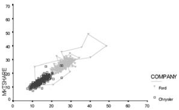
Figure 5 Phase space showingChrysler and Ford performance
Figure 5 shows the phase space diagrams for Chrysler and Ford together. The triangles represent Ford's market share change; a line connects these symbols. The open squares represent Chrysler's market share change: these symbols are not connected. There is an overlap in Ford's and Chrysler's market share performance only during the time period earlier noted. This occurs during the time period in which the most variation occurred (late 1970 to early 1971), described earlier.
Figure 6 shows the phase space diagrams for Ford and General Motors together. The triangles represent Ford's market share change; these symbols are not connected. The open circles represent General Motors' market share change; a line connects these symbols. Once again, there is an overlap in Ford's and General Motors' performance in market share only during the time period in which the most variation occurred (late 1970 to early 1971), described earlier.
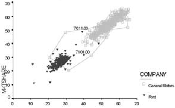
Figure 6 Phase space showing General Motors and Ford performance
The use of nonlinear research representation methods provides an important complement to traditional research representations. For example, Table 1 provides means and standard deviations for the dependent variable, market share, used in this study. The lag phase space diagrams supplement this information on variation by making changes in the dependent variable, and providing more information on the timing of variation in the system. For example, the numbered points (e.g., 7011) in the figures provide information on the timing of greatest changes in the system, which stands out from the attractor region. This information would be harder to see in a more traditional diagram of performance across time. This depiction of time also provided clues for further exploration of the source of such disturbances. A more thorough investigation of the causes of such fluctuations in market share may allow organizations to minimize the negative effects and maximize the positive effects of disturbances to the system's behavior.
DISCUSSION
The relative market share of the four companies in the US automobile industry has been shown to be stable during the time period investigated. This is consistent with the findings of other research on this industry conducted with more traditional research methods. For example, the yearly sales positions of companies in the US automobile industry (i.e., Chrysler, Ford, and General Motors) have been shown to be consistent across time using time-series analysis. The actual sales of these companies fluctuated, but their relative position remained constant: General Motors remained first, Ford second, and Chrysler third across a 25-year period (Svyantek & DeShon, 1992). Thus stability, one of the defining characteristics of an attractor (Hastings et al., 1993), may be seen in the lag phase space diagrams used here.
Organizations in mature industries exist in stasis. Stasis does not imply failure to adapt (Gould, 1993). Rather, stasis implies good adaptation to relatively constant environmental conditions across time (Bak, 1996). This adaptation, however, does not lead to radical new forms of competing (Gould, 1993) or to changes in the relative fitness of the competitors within an industry (Bak, 1996).
An important question to answer is why this stability is present. We propose that the answer is because the US automobile industry forms a complex adaptive system (CAS). The CAS is another nonlinear concept helping to explain why an industry that, to the naïve observer, embodies both the biggest and most competitive industry in the US may attain such stability.
COMPLEX ADAPTIVE SYSTEMS AND THE US AUTOMOBILE INDUSTRY
Complex adaptive systems (CAS), a major branch of complex systems theory, may be defined as systems in which agents interact with each other in different ways to form coherent, self-reinforcing clusters (Waldrop, 1992). To a layperson, a CAS is characterized by spontaneous selforganization. However, the originator of the term, Ilya Prigogine, defined self-organization as organization that arose due to the presence of a container (cf. Nicolis & Prigogine, 1989). The agents within a CAS may actively seek to turn environmental events to their advantage (e.g., in human social behavior) or passively react to stimuli (e.g., in the accumulated snow that has the potential to become an avalanche). The key is that coherent, recurring patterns of system behavior arise as the agents within the interacting cluster comprising a CAS react to or cooperate and compete among themselves.
While it is not clear that the US automobile industry has enough individual agents to constitute a CAS, the representation methods associated with CAS studies may be useful in developing a better understanding of the industry. The individual agents are the four companies (American Motors, Chrysler, Ford, and General Motors) making up the industry.
Stasis arises through the creation of a stable, integrated ecological network in which individual agents compete for resources (Bak, 1996). The agents' fitness is determined by the continuance of this network and the average fitness of individual agents in such a cluster remaining fairly constant across time. Agents do adapt, but this adaptation does not change their average fitness level.
In effect, continual adaptation by agents maintains their relative position within the network and creates a stable network of agents. The description of the US automobile industry offered here shows how entire industries may develop a homeostatic equilibrium. Each individual company has developed an attractor that defines its characteristic performance level. These attractors become resistant to perturbations (punctuated equilibrium), resulting in stasis over time.
This type of adaptation is analogous to that described for biological evolution as the “Red Queen” effect, for example VanValen (1973) and Bak (1996). The Red Queen is a character in Lewis Carroll's Through the Looking Glass. The passage reads:
“Well in our country,” said Alice, still panting a little, “you'd generally get to somewhere else—if you ran very fast for a long time as we've been doing!”
“A slow sort of country!” said the Queen. “Now here, you see, it takes all the running you can do, to keep in the same place.”
A potential explanation for this “running in place” may be found in work on competence-enhancing and competence-destroying technologies (Anderson & Tushman, 1990; Anderson & Tushman, 1991; Tushman & Anderson, 1986). Competence-destroying technological changes are typically begun by new firms and may lead to the creation of new industries or replacement of the companies comprising an existing industry (Tushman & Anderson, 1986). Competence-enhancing technological changes, on the other hand, are initiated by existing companies and do not result in such drastic changes in the industry. Competence-enhancing technological changes are more associated with established, mature industries.
The technological and product changes seen in the US automobile industry seem to be best described as competence-enhancing technological changes. They have been fairly small and incremental during the time period investigated in this study.
It has been hypothesized that the lack of innovation in most mature, established companies is due to the need to allocate resources to competition behavior with rivals in the same industry and to avoid losses due to experimentation or risk taking (Svyantek & Hendrick, 1988). For example, leaders within the automobile industry are constrained by this need not to lose against competitors (Svyantek & DeShon, 1992). This leads to the imitation of others in an industry in order to survive (Gordon, 1991). The result is that established companies in mature industries avoid risks that might offer the chance of exceptional returns. A pattern of incremental changes imitated by competitors becomes common within an industry and such advances do not offer sustained competitive advantage. This is because an advance by one company (e.g., the development of the minivan at Chrysler or the use of airbags) is easily and quickly imitated by other companies in the industry.
It may be that the starting point for a technological or product change by one agent in the system is the desire to create a competence-destroying change. The development of the minivan during the period of investigation might be one such change. Chrysler may have hoped that this development would lead to a change in its relative position in the US automobile industry. The key, however, is the reactions of the other agents in the system to a change. Here, Ford and General Motors quickly imitated Chrysler and developed their own minivans. If such imitation occurs, the change is competence enhancing, despite the original intentions of its developer.
An interesting hypothesis is that the agent with low performance is most likely to be innovative. As noted, Chrysler, the smallest and least profitable of the Big Three in the US automobile industry, was responsible for the development of the minivan. It may be that the risks associated with the development of such new products may only be justified if an agent is not performing as well as others. Unfortunately, such innovations are easily imitated by other agents. These imitations may eventually outperform the original innovation (e.g., the Ford Windstar now outsells Chrysler minivans). But until a clear niche for the product is defined, the more effective agents (Ford and General Motors here) need not be innovative because they are already outperforming other agents.
This proposal that innovation occurs in the least effective performers is supported by two recent developments. First, the same process is occurring for a recent product development after the time period investigated in this study. Chrysler recently introduced the PT Cruiser, a model with retro styling. It was an immediate hit with the American public. Less than two years after the introduction of this model, Ford and General Motors are introducing their versions of cars designed to attract the same buyer (Duarte, 2001; Howes, Miller, & Truby, 2001). Whether or not these models will outsell the original Chrysler model is a matter for the future to decide. But the innovation came from Chrysler, which was still the lowest performing agent. Further support for the proposal is that technically Chrysler, as of 1998 and its acquisition by Daimler-Benz, is no longer truly a member of the US automobile industry
The “Red Queen” effect is interpreted here as describing the process through which the companies in the US automobile industry continually adapt but are only able to maintain, not improve, their places in their market. Adaptation, therefore, does not mean more successful performance: It only means staying in the game.
The results of this study support the premise that the US automobile industry has undergone long periods of stasis in which the relative fitness and position of its members do not change in phase space.
One explanation for the results of this study may be found in the literature on the relationship between organizational culture and corporate performance in organizations. Barney (1986) has proposed that organizational culture is seldom a source of sustained financial value to a company. To provide a sustained competitive advantage, the culture of an organization must allow the firm to do things that add value to its output; be rare in relation to the cultures found in competitor firms; and be imperfectly imitable by other firms in the same industry.
The degree to which an innovation by one company is imperfectly imitable is probably less than typically believed. Davis (1984) states that organizational cultures reflect both a company's orientations toward the management of internal human resources and how they compete against external competitors. Gordon (1991) has suggested that the formation of these two orientations within any company is dependent largely on industry-wide assumptions about customers, competitors, and society. Organizations in the same industry will use similar procedures to implement similar strategies derived from these assumptions. CEOs will be constrained by the cultures in which they develop and reside (cf. Tushman & Romanelli, 1985). Therefore, the succession of CEOs within an industry is not a guarantee of any influence from new ideas, because the cultures of the two intra-industry companies will share similar assumptions. For example, a longitudinal analysis of the performance of Ford and Chrysler after Lee Iaccoca's move from one to the other showed little effect on the overall performance of the two companies (Svyantek & DeShon, 1992). The US automobile industry appears to be particularly susceptible to the development of similar assumptions across companies (Abrahamson & Fombrun, 1994).
These shared assumptions form a macro-culture (Abrahamson & Fombrun, 1994). Macro-cultures increase the degree to which companies in an industry are innovative. They increase the likelihood that members of the same industry will have similar strategic profiles. It can be posited that members of an industry come to react to environmental change in the same way.
The stasis seen in the system described here is attributable to the development of a macroculture within the US automobile industry. Innovation occurs within bounds set by the macroculture no matter which individual agent is making the innovation. The other agents in the system, therefore, are able readily to imitate the change. The net result is the lack of change in relative position among the agents in the system when performance is assessed across time.
CONCLUSIONS
This study has shown that nonlinear research representation methods (lag phase space diagrams) may be used to investigate change in organizational criteria across time. The use of the lag space diagrams showed that attractor regions for the performance of the companies comprising the US automobile industry can be found and illustrated. It was proposed that these attractors represent the relative fitness of each company in the industry. The relative positions were in stasis during the 27-year period investigated here, since each company maintained a relatively fixed position in terms of market share across time. Potential reasons for the maintenance of the relative position of the companies across time were discussed. It was hypothesized that the companies formed a complex adaptive system, and that this CAS was defined by a macroculture setting boundaries on the degree to which innovation might occur in the industry. While this explanation is doubtlessly incomplete, it does provide a picture with which to view both the industry and policy making with regard to that industry.
The use of nonlinear research representation methods provides an important complement to traditional research representations. A recent study by Svyantek and Snell (1999) illustrates this. It evaluated the effects of an organizational intervention across a three-year period in six plants of one organization. Three plants had a gainsharing intervention put in place to increase performance, while three plants used a fixed bonus system to reward productivity. The question of interest to the company's management was which incentive program worked better. Traditional statistical analyses showed no between or within group differences across the two groups of plants for the first two years of the intervention. The gainsharing intervention was continued because the company management perceived that things were getting better, although no statistical proof was found. Svyantek and Snell used lag phase space diagrams to represent the results of the intervention. These representations showed that there was a drastic decrease in performance variability for the three plants receiving the gainsharing intervention from the first to second year. This continued into the third year. The representations found using nonlinear research methods were interpreted as providing supplementary information to the evaluation of change in organizations.
Policy makers looking at organizational problems gain from the inclusion of the representations derived from nonlinear research methods. These statistical graphing techniques allow the representation of change and the relationship among variables to be pictured. The use of nonlinear research representation methods provides a new, complementary perspective for looking at organizations. This perspective emphasizes the temporal dimension of a system's behavior. The understanding offered by taking a complex adaptive system approach requires a more in-depth understanding of the historical processes and interactions that lead to the development of consistent patterns of behavior across time. The study of organizations (and social systems in general) as complex adaptive systems requires that researchers take a much more longitudinal, historical, and in-depth, context-specific approach. Taking such an approach, however, offers an exciting new way to describe organizations and organizational attractors and provides insight for the improvement and/or change of these attractors.
NOTE
The research reported in this study was supported by a Faculty Research Grant from The University of Akron.
References
Abraham, F. D., Abraham, R. H., & Shaw, C. D. (1990) A Visual Introduction to Dynamical Systems Theory for Psychology, Santa Cruz, CA: Aerial Press.
Abrahamson, E. & Fombrun, C. J. (1994) “Macrocultures: Determinants and consequences,” Academy of Management Review, 19: 728-55.
Anderson, P & Tushman, M. L. (1990) “Technological discontinuities and dominant designs: A cyclical model of technological change,” Administrative Science Quarterly, 35: 604-33.
Anderson, P & Tushman, M. L. (1991) “Managing through cycles of technological change,” Research Technology Management, 34: 26-31.
Ayers, S. (1997) “The application of chaos theory in psychology,” Theory and Psychology, 7: 373-98.
Bak, P (1996) How Nature Works: The Science of Self-Organized Criticality, New York: Copernicus.
Barney, J. B. (1986) “Organizational culture: Can it be a source of sustained competitive advantage?,” Academy of Management Review, 11: 657-65.
Briggs, J. & Peat, F. D. (1989) Turbulent Mirror: An Illustrated Guide to Chaos Theory and the Science of Wholeness, New York: Harper & Row.
Carroll, L. (1899) Alice's Adventures in Wonderland and Alice Through the Looking Glass, Chicago: Donohue & Henneberry.
Davis, S. M. (1984) Managing Corporate Culture, Cambridge, MA: Ballinger.
Duarte, J. (2001) “Imitation is the sincerest form of flattery,” Toronto Sun, February 18: D18.
Gleick, J. (1987) Chaos: Making a New Science, New York: Viking.
Gordon, G. G. (1991) “Industry determinants of culture,” Academy of Management Review, 16: 396-415.
Gould, S. J. (1993) “The inexorable logic of the punctuational paradigm: Hugo de Vries on species selection,” in D. R. Lees & D. Edward (eds), Evolutionary Patterns and Processes, London: Academic Press: 3-18.
Hastings, A., Hom, C. L., Ellner, S., Turchin, P, & Godfray, H. C. J. (1993) “Chaos in ecology: Is Mother Nature a strange attractor?,” Annual Review of Ecology and Systematics, 24: 1-33.
Howes, D., Miller, J., & Truby, M. (2001) “Auto firms hunker down: Detroit touts niche products at Cobo to boost sagging prices,” Detroit News, January 7: A1.
Hutcheson, G. D. & Hutcheson, J. D. (1996) “Technology and economics in the semiconductor industry,” Scientific American, 274: 54-63.
Kellert, S. H. (1993) In the Wake of Chaos: Unpredictable Order in Dynamical Systems, Chicago: University of Chicago Press.
Kiel, L. D. (1996) “Nonlinear dynamical analysis: Assessing systems concepts in a government agenc,” in J. M. Shafritz & J. S. Ott (eds), Classics of Organization Theory, Belmont, CA: Wadsworth Publishing: 592-606.
Liebovitch, L. S. (1998) Fractals and Chaos Simplified for the Life Sciences, New York: Oxford University Press.
Nicolis, G. & Prigogine, I. (1989) Exploring Complexity: An Introduction, New York: W. H. Freeman.
Savit, R. (1991) “Chaos on the trading floor,” in N. Hall (ed.), Exploring Chaos: A Guide to the New Science of Disorder, New York: W. W. Norton: 174-83.
Svyantek, D. J. (1997) “Order out of chaos: Non-linear systems and organizational change,” Current Topics in Management, 2: 167-88.
Svyantek, D. J. & Brown, L. L. (2000a) “Complex systems and the measurement of organizational change,” Current Topics in Management, 5: 41-62.
Svyantek, D. J. & Brown, L. L. (2000b) “A complex-systems approach to organizations,” Current Directions in Psychological Science, 9: 69-74.
Svyantek, D. J. & DeShon, R. P (1992) “Leaders and organizational outcomes: An analysis of Lee Iaccoca and the American automobile industry,” in K. E. Clark, M. B. Clark, & D. C. Campbell (eds), Impact of Leadership, Greensboro, NC: Center for Creative Leadership: 293-303.
Svyantek, D. J. & DeShon, R. P (1993) “Organizational attractors: A chaos theory explanation of why cultural change efforts often don't,” Public Administration Quarterly, 17: 339-55.
Svyantek, D. J. & Hendrick, H. L. (1988) “The nature of change: An extension of new developments in evolutionary theory to the study of organizational systems,” Proceedings of the Annual Human Resource Management and Organizational Behavior Meetings, I: 243-47.
Svyantek, D. J. & Snell, A. S. (1999) “Knowledge out of chaos: Using phase spaces for the qualitative evaluation of organizational change,” in M. P Cunha & C. A. Marques (eds), Readings in Organization Science: Organizational Change in a Changing Context, Lisboa, Portugal: Instituto Superior de Psicologia Aplicada: 523-40.
Tushman, M. L. & Anderson, P (1986) “Technological discontinuities and organizational environments,” Administrative Science Quarterly, 31: 439-65.
Tushman, M. L., & Romanelli, E. (1985) “Organizational evolution: A metamorphosis model of convergence and reorientation,” Research in Organizational Behavior, 7: 171-222.
VanValen, L. M. (1973) “A new evolutionary law,” Evolutionary Theory, 1: 1-30.
Wainer, H. & Velleman, P F (2001) “Statistical graphing: Mapping the pathways of science,” Annual Review of Psychology, 52: 305-55.
Waldrop, M. M. (1992) Complexity: The Emerging Science at the Edge of Order and Chaos, New York: Simon & Schuster.