Introduction
In the ‘information age’ there is a general belief that having access to as much information as possible is a good thing, leading to more effective decision making and thus allowing us to rationally design the world in our image. Of course, any sophisticated view of the information age has to acknowledge that having information for the sake of information is not much more useful than having no information. What is key is having access to the right information at the right time, where knowing both what is the ‘right’ information for the ‘right’ time are highly problematic assessments. We are slowly beginning to acknowledge that in a complex world, ‘states of affairs’ much be considered from multiple directions whilst maintaining a (constructively) critical disposition at the same time. This comes about because the external concrete reality we perceive is not quite as solid as our more recent scientific heritage would suggest. The relationship between our universe and our understanding of it is, dare I say it, very complex.
Along side this popular belief that information should be abundant and freely available, is that being connected is also the preferred state of existence. Like all ideas, ‘being connected’ has limits to its usefulness. Is there a preferred degree of connectedness? An individual who was not connected at all could achieve nothing. Indeed, without some degree of connectedness, an individual could not even be recognized as such - we are, to a large extent, defined by our connections. At the other end of the spectrum, if an individual is too connected then it becomes also most impossible to achieve anything coherent. If too much is going on at once, and no stable patterns emerge (even if only temporarily) then again the notion of the individual and his/her identity is impossible to discern - the whole system becomes the only useful unit of analysis.
This short discussion article represents an early report into some research I have been performing that explores the relationship between connectivity and system behavior. The area I will be focusing upon herein is how a system’s behavior develops as more and more inter-connections are added between individual system components. As in other articles I have written for E:CO (Richardson, 2004a, 2004b, 2005a) I will be using Boolean networks to explore this behavior. As I have suggested before, although Boolean networks are probably too simple to represent social reality in any complete sense, I believe that the lessons that can be learnt are still valid (albeit with some contextual restrictions) for more complex systems. I also tend to believe that some of the more general conclusions that can be drawn from the exploration of such systems are largely obvious. However, such models allow us to explore these behaviors scientifically rather than develop purely from the wisdom that comes with considerable experience. Even if science confirms what we think we already know, science allows us to investigate more thoroughly and rigorously our ideas in ways that more often than not lead to an enrichment in our understanding (especially if we can avoid getting too hung up on particular paradigms!).
Basic parameters
I do not plan to go into great detail about Boolean networks and how they are constructed and simulated. The interested reader might read Lucas (2007), or Richardson (2005b). In this section I want to introduce a number of parameters that can be used to characterize the phase space of complex systems (Boolean networks in particular). I hope that after 8½ volumes of E:CO I do not need to spend time defining concepts such as ‘phase space’ and ‘attractors’ in detail. For the purposes of this article I would like to briefly describe the following measures:
Number of attractors, 1. Natt;
The weight of the largest attractor as a per2. centage of the total size of phase space, Wmax;
The maximum number of pre-images for a 3. particular network configuration, PImax;
The longest transient for a particular net4. work, Tmax;
The number of Garden-of-Eden states as a 5. percentage of the total size of phase space, G.
The average robustness for a particular net6. work, R;
Phase Space Attractors
The number of phase space attractors is probably the most single important characteristic of a nonlinear dynamical system. In Boolean networks, all trajectories end up (after some transitory period) on periodic attractors. Given that Boolean networks are discrete networks one would never observe the type of chaotic behavior as seen in certain continuous systems. However, attractors with periods much larger than the size of the network are often referred to as quasi-chaotic or quasi-random. Indeed, it is a relatively trivial task to create Boolean networks that contain attractors with periods so large that for all intents and purposes (and by all standard tests of randomness) they are random. The primary interest in the number of attractors displayed by a particular network, is that this number corresponds directly with the number of qualitatively different behavioral modes that particular network can operate in. So, if a network only exhibits a single attractor then it only has one function. If it has many then it has many functions. This is overly simplistic of course. As we shall see, networks with huge numbers of attractors (as compared to the size of the network itself) are not very connected, and so they can easily be reduced to a number of independent (non-interacting) sub-networks that do not display very interesting behavior. The behavior of such networks can easily be explained analytically, i.e., with some quite simple mathematics. At the other extreme, are highly connected networks that exhibit few attractors that do behave in an interesting manner not easily considered from an analytical perspective, such is the nature of nonlinear dynamics. We shall explore how connectivity and the number and type of attractors relate to each other later in this article.
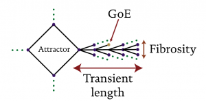
The attractors themselves generally only contain a small percentage of the number of states comprising the network’s complete phase space (2N). The remaining states describe trajectories from arbitrary points in phase space to particular attractors. The set of all attractor states and the states that comprise the various trajectories to a particular attractor form an attractor basin. The proportion of the total number of states comprising state space that comprise a particular basin is referred to as the basin’s relative weight. An idealized attractor
An?idealized?attractor?basin
Pre-images
Although, for Boolean networks, the application of the rule table results in only one unique state (the networks are forward deterministic), reversing this algorithm may lead to more than one solution, i.e., any particular state may have more than one state that leads to it (so Boolean networks are not backward deterministic). A high average pre-image number results in fibrous-looking branches flowing to the central attractor. As such for the remainder of this article I will refer to average pre-image number as fibrosity, or F. Another important parameter is maximum transient length.
Maximum transient length
The maximum transient length, Tmax, is essentially a measure of the furthest distance one can get from the central attractor by applying the rule-based algorithm backwards. Let’s say a network is started from a state that is ten states away from the central attractor. Once the network is simulated, it will take ten time steps before the central attractor (associated with the starting state) is reached. We might also refer to this transitory period as the network’s settling time. If we assume that, in the real world, there is some degree of uncertainty in pushing a network to a particular state so that it adopts a particular mode of behavior, then (assuming we are even able to select a state on the correct basin) there will be a delay between the intervention and the desired (hopefully) response. There may in fact be a relatively long delay between the intervention and the network adopting the desired mode of operation, so long in fact, that it can be make the connection between cause and effect difficult to determine. (And, this of course ignores the possibility that another intervention doesn’t nudge the system towards another basin in the meantime). So long settling times are problematic for the intervener.
As phase space is finite, if settling times are long then fibrosity is relatively low. At one extreme we have short fibrous attractor branches that ensure that the central attractor is reached quickly from many possible starting points. At the other extreme we have long sparse attractor branches that can result in significant delays between action and desired response (although the system will respond immediately by following a trajectory toward the characteristic attractor).
Gardens-of-Eden
Figure 1 also indicates a state labeled ‘GoE’ which is shorthand for ‘garden-of-eden’. Mathematically, when rolling back time to construct these attractor basins a point is eventually reached for which there is no solution. These states cannot be reached from any other states—they are, in a sense, the beginning of time for the particular trajectory they ‘create’—hence, the reference to the Garden of Eden (see Wuensche & Lesser, 1992; Wuensche, 1999). From a control perspective, internal mechanisms do not have any capacity to access GoEs—for all intents and purposes they do not exist, from an internal viewpoint. However, they can be reached from the outside by perturbing the network in a way that forces it to adopt a GoE state (from there the network will follow the trajectory that that state ‘creates’, although note that the particular trajectory will comprise states that are accessible from the inside). The practical upshot of the existence of GoEs is simply that if an external intervener (or, ‘perturber’) wanted to encourage the network towards a particular attractor s/he/it would have more states available to initiate the desired response. Of course, to take full advantage of this benefit the external intervener would have to have perfect knowledge of the network’s phase space. In the absence of such absolute understanding, it still follows that an external intervener can potentially ‘see’ more of the network’s phase space, than an internal intervener can, and arguably has a greater variety of maneuvers that s/he/it can execute to achieve designed ends.
Dynamic robustness
I have already suggested that the number of phase space attractors is one of the more important attributes of a dynamic system. However, although two states may be next to each other on an attractor basin (i.e., in phase space), they may in fact be very far from each other in state space. For example, in a very small network containing only five nodes the state 00001 and 00010 are next to each other in state space, but in phase space they might actually lie on different attractor basins. As such, in order to have a better appreciation of a system’s dynamics we need to understand how the states on a particular attractor basin are distributed across state space. We shall see such a state space portrait later on, but for now I want to consider a measure that takes into account both phase and state space structure. Dynamic robustness, R, is a measure of the chances of pushing a network into a different basin with a small nudge. In the case of Boolean networks, R for single state is calculated by adding together the total number of 1-bit perturbations that do not result in a switch to a different basin, and dividing this number by the size of the network, N. For example, if we consider a network of size N=5 and the state 00010 then there are five 1-bit perturbations: 10010, 01010, 00110, 00000, 00011 (the emboldened state is the reversed one). If three of these give states lie on the same basin then the dynamic robustness of state 00010 is 3/5. The network’s overall dynamic robustness is simply the average of all the values of R for a single state. If R is high, say > 80%, then the network’s qualitative behavior is relatively stable in the face of small external perturbations. If R is low, say < 20%, then the majority of small external signals will result in a qualitative change in behavior. The dominant factor in this measurement is of course the number of attractors, but the distribution of the states lying in a particular basin also affects the overall measurement.
In one sense the total number of attractors is equivalent to the number of contexts, or environmental archetypes, a system ‘sees’ and can respond to. As with many of the measures presented here, there is a balancing act to be performed. If a network ‘sees’ too many environmental archetypes, then it is essentially at the beck and call of the environment. If it ‘sees’ only one archetype, i.e., phase space is characterized by only one attractor basin, then the network has no variety in its responses to environmental changes whatsoever.
However, dynamic robustness also has an effect on a network’s ‘sight’. Dynamic robustness can be high if the states associated with each basin are distributed in such a way as to maximize R for a particular number of basins (this is more likely when no one basin is significantly heavier than the others). However, networks that are characterized by many basins may also exhibit high dynamic robustness if one of those basins is considerably larger (heavier) than the others. In this latter situation, although the network has the potential to ‘see’ and respond to many environmental archetypes, it overly privileges one particular archetype and so effectively blinds itself to others.
The heart of this article is concerned with how the various parameters presented above vary with increasing network connectivity, but before moving on to consider these relationships a brief presentation of the computer experiment performed will be given.
Growing Boolean networks
The computer experiment performed for this study starts with a network of N=15 nodes that contains no interconnections whatsoever (by most standards this starting point would not even deserve the label ‘network’). In order to simulate a Boolean network, associated with each node is a rule table that determines what state a particular node will acquire on the next time step which is dependent upon the state of its input nodes for the current time step. For the starting point (completely disconnected nodes), each node simply maintains the same state from time step to time step (in essence there is no rule table, only the rule that the state of the node does not change over time). This results in 2N point attractors that have no transient branches whatsoever (attractor weight = attractor basin weight = 1 state). Once the number of attractors and their branch structure have been determined, a connection is added between two randomly selected nodes (with the proviso that no connection already exists between those two random selected nodes). Once connections are made a process for evolving a node’s rule table is required. For this study the following example illustrates the algorithm that was used.
The number of input combinations that a single node can respond is 2k, where k is the number of inputs. For example, for a node with k=2 inputs there are four possible input configurations. The rule table for such a node may look like:
The rule for a node with this response configuration can be expressed simply as 0110. Now let us consider that the node has now acquired another input with node C. There are now 23 = 8 possible input configurations. For the algorithm used herein, when the state of node C is 0 (or off), the response to A and B is kept the same as it was before the connection from node C was added. The response to the additional four configurations that are formed when the state of node C is 1 (or on) are selected randomly. So,
Simply expressed the rule changes from 0110 to 11000110 (where the emboldened digits represent the ‘old’ rule). As the number of connections, C, are increased the rule for a particular node may evolve as:
C Rule
1 10
2 0110
3 11000110
4 0110011011000110
5 11010001101011000110011011000110
Etc.
When the network is fully connected (C = 210 = N[N-1]) the rule for each node is represented by a string containing a sequence of 214=16384 ‘0’s and ‘1’s (note that connections to self are not included) with the basic structure illustrated above. The value of each parameter was determined as each additional connection was made. This process was repeated 1000 times and the results averaged across this sample set. The results of this computer experiment will presented and discussed next.
Experimental results and discussion
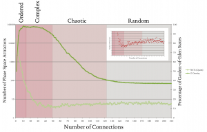
N A and GoEs
Figure 2 shows the relationship between the number of phase space attractors, NA, and the percentage of GoEs with the number of connections, C. There are four distinct regions. The first region shows the number of attractors decreasing rapidly and the proportion of GoEs increasing rapidly. The rapid decrease in NA is due to the fact that as each new connection is made NA is halved. This is not always the case, but the important characteristic of this ‘ordered’ region is that the qualitative structure of phase space can easily be determined analytically. This is because in this region of low-C, no interacting feedback loops are formed amongst the interconnections.
The second region, which is labeled ‘complex’ sees a continued decrease (although at a much slower rate than in the ordered region) in the number of attractors, down to a minimum of around four attractors. The proportion of GoEs is also constantly high throughout this region, indicating that the vast
The?relationship?between?network?connectivity?and?number?of?phase?space?attractors?/?percentage?of?Garden-of-Eden?states
The next region, termed ‘chaotic’, is characterized by a steady and relatively rapid drop in the proportion of GoEs, from around 97% to 40%, and a slow rise in the number of attractors from approximately four to six. It is difficult to say much about this region without calling upon other data (which we will do shortly), other than there is a significant increase in states that are not only accessible from outsidethe system. The same is true for the last region—‘random’—for which the number of attractors and the proportion of GoEs remain relatively steady at six and ~40%, respectively.
R and Wmax
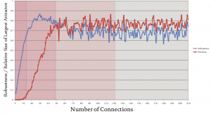
Figure 3 shows the relationship between network connectivity, C, and both dynamic robustness, R, and the weight of the largest attractor basin, Wmax, i.e., the basin containing the most states. In the ‘ordered’ region there is a rapid increase in dynamical robustness that is attributable to the rapid decrease in the number of attractors (shown in Figure 2). Also of note is the very low weight of the ‘heaviest’ basin, which again is the result of the large number of attractors characteristic of networks in this region.
The?relationship?between?network?connectivity?and?dynamic?robustness?/?relative?size?(weight)?of?the?largest?(heaviest)?attractor
The ‘complex’ region is where it all happens within this particular dataset. The weight of the heaviest basin increases rapidly, and the dynamical robustness increases to 0.85 (at C?2N) before decreasing rather slowly to ~0.70. The rapid increase in Wmax can be interpreted as an increase in archetypal preference—across this region the networks’ behavior changes from having little preference for a particular mode of behavior (which means they ‘see’ many types of environmental context—indicatory of a relatively large number of attractors), to having a definite preference to the mode of behavior they exhibit (which means they are ‘tuned’ to one particular environmental context). Another way of expressing this shift is that the networks go from being overly flexible to being overly inflexible and that in the middle of the complex region there is a balance between qualitative pluralism and monism (or, dogmatism).
There is little to distinguish the ‘chaotic’ and ‘random’ regions in this particular dataset. Both R and Wmax are relatively stable at 0.70 and 0.75, respectively, suggesting that the phase spaces of networks existing in these regions are dominated by a single heavy attractor basin.
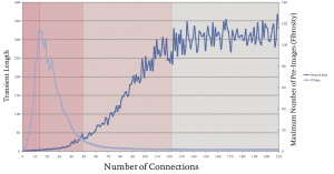
Fibrosity and settling time
Figure 4 shows the relationship between network connectivity, C, and both PImax (or, fibrosity) and Tmax (transient, or settling time). If we consider the ordered region first then we observe that over this region fibrosity increases rapidly to a maximum of around 110, whilst at the same time, the maximum settling time remains very low. This indicates that whatever state a network in this region is initiated from, the trajectory will reach an attractor very quickly (bearing in mind that these attractors will be rather uninteresting as they are analytically trivial).
In the ‘complex’ region we see a rapid decrease in fibrosity along with a modest increase in maximum settling time1. The phase space of the average network in this region,
The?relationship?between?network?connectivity?and?transient?length?(settling?time)?/?maximum?number?of?pre-images?(fibrosity)
The ‘chaotic’ and ‘random’ regions, which contains networks whose phase space is dominated by a single heavy attractor, are distinguished by the quite different structure of the branches attached to the states on the central attractor. ‘Chaotic’ branches tend to be quite long and quite fibrous, whereas ‘random’ branches tend to be very long and sparse.
Now that we have considered each of the datasets separately, we can move on to constructing the ‘bigger picture’ by considering all the datasets together and developing a fuller appreciation of each network type. Before doing that, however, I want to highlight that the regional denotations presented herein relate to the characteristic networks’ dynamics and not necessarily their structural topology (although connectivity is an important structural parameter). Network theorists distinguish between ordered, small-world, scale-free and random networks. These structural denotations do not map directly to the dynamic denotations of ordered, complex, chaotic and random. For example, the (dynamically) ‘random’ that we shall see in the next section is far from random from a structural perspective. That being said, an interesting area for investigation, especially in the ‘complex’ region, would be how the dynamic structure (i.e., emergent modularity) maps to phase space structure.
Considering all the data sets as one
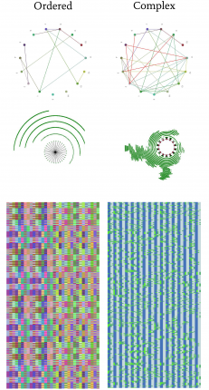
Table 1 attempts to sum-up the observations made in the previous sections, by showing how each parameter changes qualitatively (e.g., ??? = rapid increase) over each region. Figure 5 brings presents the data visually (and arguably more effectively) by comparing the network structure, the largest phase space attractor basin, and the state space configuration (the online PDF version of this article is recommended so that full color can be observed) for a ‘typical’ network selected from each region. Figure 5 vividly illustrates the differences in attractor basin structure and state space configuration and allows us to see directly the impact that parameters such as fibrosity and robustness have on these two ‘spaces’.
Part?1
Structural topology, the largest phase space attractor basin, and the state space configuration for an ordered and a complex network
Part?2
Structural topology, the largest phase space attractor basin, and the state space configuration for a chaotic and a random network
Table?1
Qualitative change in principle parameters across each dynamic region
| Network Type | Natt | PImax | Tmax | GoE | R | Wmax |
|---|---|---|---|---|---|---|
| Ordered | ??? | ??? | ? | ??? | ??? | ? |
| Complex | ?? | ??? | ?? | ? | ? | ??? |
| Chaotic | ? | ? | ??? | ?? | ? | ? |
| Random | ? | ? | ? | ? | ? | ? |
Missing data: Pmax
P max refers to the period of the heaviest (Wmax) attractor basin for a particular network. This additional data would be useful as the case of Pmax » N is often used to justify the term ‘chaotic’ for a Boolean network. A full analysis of how Pmax varies with C was not available at the time of writing, but early indications show that Pmax increases with C. This trend is illustrated (amongst others) in Table 2 which reports the values of the Pmax, and the other parameters discussed thus far, for the four networks depicted in Figure 5. This very small sample confirms that the period of the heaviest basins (Pmax) for typical networks in the ‘chaotic’ and ‘random’ regions are indeed much larger (») than the network size (N).
We can now attempt to make a ‘standard’ statement about each of the four dynamic regimes: ordered, complex, chaotic and random. It should be noted, however, that the statements that follow are of the ‘on average’ variety, in that there will exist networks in each region that look (in a dynamic sense) very much like networks in other regions. A more obvious limitation of such a categorization process is that the boundaries between each region are fuzzy and certainly not discrete. The statements are, therefore, no more than guidelines. They certainly do not allow us to make statements of the sort “All Boolean networks with N=15 and C=60 are dynamically chaotic.” Although statements such as “Networks with N=15 and C=60 (with the same rule structure discussed herein) typically display dynamic traits that resemble chaotic behavior” are meaningfully efficacious. As with all of complexity thinking (and arguably all science and even all human thinking) we must resist the temptation is creating hard rules from fuzzy guidelines—guidelines need to balance the need to say something meaningful, without saying too much. To state this differently, one might also suggest that “to say something meaningful about complex systems, one must also be a little vague.” The following characteristic statements illustrate this:
A dynamically ordered network responds to many environmental changes quickly and without preference. The various behavioral modes available to the network are analytically trivial. Once in a particular mode, such networks are quite susceptible to external perturbations. Furthermore, a modest number of states can only be accessed from outside the system.
A dynamically complex network responds quite quickly to a modest number of environmental changes with some degree of preference. The various behavioral modes available to these networks are analytically irreducible and innovative. Once performing a particular function, such networks are very robust to external perturbations. Furthermore, a high number of states can only be accessed from outside the system.
A dynamically chaotic network responds rather slowly to a modest number of environmental contexts, but with a high preference for one particular archetype. The dominant mode is very complex to the point of being chaotic. Such networks are very robust to external signaling and a significant number of states can only be accessed from outside the system.
A dynamically random network responds very slowly to a modest number of environmental contexts, but with a high preference for one particular archetype. The dominant mode is very complex to the point of being chaotic. Such networks are very robust to external signaling and yet only a low proportion of states can only be accessed from outside the system.
The emboldened terms are relative assessments that only gain meaning through comparison with the other types. We go even further with this process of data reduction. Consider the following slogans:
Ordered = fast, fickle and predictable;
Complex = swift, balanced and inventive;
Chaotic = sedate, dogmatic and incoherent;
Random = slow, stubborn and unfocused.
The more ‘distance’ however between the raw data and our summations, the more subjective dimensions play in our choice of words. For example, if a different slant was taken we might rewrite the slogan for chaotic as:
Chaotic = Thorough, strong-willed and sophisticated.
My point is simply that the process of categorizing complex datasets is problematic and requires a great deal of care.
Final remarks
The motivation for this article was to explore the merits of a modern assumption that ‘being connected’ is unquestionably a good thing. The research presented here is still in its early phases, but it is clear that different levels of connectivity can be associated with different types of dynamics. One interpretation would suggest that being too connected is actually overly restrictive and that there is a balance to be maintained. Much of the complexity literature argues that “maintaining balance” is central to a sustainable approach for existing within a complex (eco-) system. Of course, we must take care in importing the lessons from abstract models such as Boolean networks into the realm of human organization. That being said, what is rather surprising to me is how narrow the desired ‘balanced’ (complex) region is relative to the (seemingly less desirable) chaotic and random regions. Furthermore, if we consider the width of the complex region, Cwidth, in relation to the whole of ‘connectivity space’ we can construct a measure of relative weight, Wcomplex, equal to the width of the complex region divided by the total number of a connections in a fully connected network. In this particular study Wcomplex ? 2N/(N[N-1]). If we take the bold (and possibly wrong!) step of assuming this is true for increasingly larger networks then Wcomplex?N-1, and so as N increases the relative width of the complex region becomes vanishingly small. Balance is achieved it seems, not by occupying ‘the middle ground’, but ‘a narrow strip of ground off to one side’!
Footnotes
[1] The fact that a large decrease in PImax is associated with only a modest increase in Tmax is simply that there are more states required to increase Tmax than PImax. If PImax increases rapidly then state space quickly runs out of available states before a phase space trajectory can get too far from the central attractor.