What Is Complexity Science?
Knowledge of the Limits to Knowledge
Peter Allen
Cranfield University, USA
Introduction
In a recent article (Allen, 2000), the underlying assumptions involved in the modeling of situations were systematically presented. In essence, we attempt to trade the “complexity” of the real world for the “simplicity” of some reduced representation.
The reduction occurs through assumptions concerning:
- The relevant “system” boundary (exclude the less relevant).
- The reduction of full heterogeneity to a typology of elements (agents that might be molecules, individuals, groups, etc.).
- Individuals of average type.
- Processes that run at their average rate.
If all four assumptions can be made, our situation can be described by a set of deterministic differential equations (system dynamics) that allow clear predictions to be made and “optimizations” to be carried out. If the first three assumptions can be made, then we have stochastic differential equations that can self-organize, as the system may jump between different basins of attraction that reflect distinct patterns of dynamical behavior. With only assumptions 1 and 2, our picture becomes one of adaptive evolutionary change, in which the pattern of possible attractor basins alters and a system can spontaneously evolve new types of agent, new behaviors, and new problems. In this case, naturally we cannot predict the creative response of the system to any particular action we may take, and the evaluation of the future “performance” of a new design or action is extremely uncertain (Allen, 1988, 1990, 1994a, 1994b). In summary, a previous article (Allen, 2000) showed how the science of complex systems could lead to a table concerning our limits to knowledge. If we now take the different kinds of knowledge in which we may be interested concerning a situation, we can number them according to:
- What type of situation or object we are studying (classification: “prediction” by similarity).
- What it is “made of” and how it “works.”
- Its “history” and why it is as it is.
- How it may behave (prediction).
- How and in what way its behavior might be changed (intervention and prediction).
We can then establish Table 1, which therefore in some ways provides us with a very compressed view of the science of complexity.
| Assumptions | 2 | 3 | 4 | 5 |
|---|---|---|---|---|
| Type of model | Evolutionary | Self-organizing | Nonlinear dynamics (including chaos) | Equilibrium |
| Type of system | Can change structurally | Can change its configuration and connectivity | Fixed | Fixed |
| Composition | Can change qualitatively | Can lead to new, emergent properties | Yes | Yes |
| History | Important in all levels of description | Is important at the system level | Irrelevant | Irrelevant |
| Prediction | Very limited Inherent uncertainty | Probabilistic | Yes | Yes |
| Intervention and prediction | Very limited Inherent uncertainty | Probabilistic | Yes | Yes |
Table 1 Systematic knowledge concerning the limits to systematic knowledge
The idea behind the “modeling” approach is not that it should create true representations of “reality.” Instead, it is seen as one method that leads to the provision of causal “conjectures” that can be compared with and tested against reality. When they appear to fit that reality, we may feel temporarily satisfied; when they disagree with reality, we can set about examining why the discrepancy occurred. This model is our “interpretive framework” for sense making and knowledge building. It will almost certainly change over time as a result of our experiences. It is developed in order to answer questions that are of interest to the developer, or the potential user, and both the model and the questions will change over time. The questions that are addressed influence the variables that are chosen for study, the mechanisms that are supposed to link them, the boundary of the system considered, and the type of scenarios and events that are explored. The model is not reality, but merely a creation of the modeler that is intended to help reflect on the questions that are of interest. The process involved is not telling us whether our current model is true or false, but rather whether it appears to work or not. If it does, then it will be useful in answering the questions asked of it. If it doesn't, then it is telling us that we need to rethink our interpretive framework, and that some new conjecture is needed.
The usefulness may well come down to a question of the spatiotemporal scales of interest to the modeler or user. For example, if we compare an evolutionary situation to one that is so fluid and nebulous that there are no discernible forms, and no stability for even short times, we see that what makes an evolutionary model possible is the existence of quasi-stable forms for some time at least. If we are only interested in events over very short times compared to those usually involved in structural change, it may be perfectly legitimate and useful to consider the structural forms as fixed. This doesn't mean that they are, it just means that we can proceed to do some calculations about what can happen over the short term, without having to struggle with how forms may evolve and change. Of course, we need to remain conscious that over a longer period forms and mechanisms will change and that our actions may well be accelerating this process, but nevertheless it can still mean that some selforganizing dynamic is useful.
Equally, if we can reasonably assume not only that system structure is stable but in addition that fluctuations around the average are small, we may find that prediction using a set of dynamic equations provides useful knowledge. If fluctuations are weak, it means that large fluctuations capable of kicking the system into a new regime/attractor basin are very rare and infrequent. This gives us some knowledge of the probability of this occurring over a given period. So, our model can allow us to make predictions about the behavior of a system as well as the associated probabilities and risk of an unusual fluctuation occurring and changing the regime. An example of this might be the idea of a 10-year event and a 100-year event in weather forecasting, where we use historical statistics to suggest how frequent critical fluctuations are. Of course, this assumes an overall “stationarity” of the system, supposing that processes such as climate change are not happening. Clearly, when 100-year events start to occur more often, we are tempted to suppose that the system is not stationary, and that climate change is occurring. However, this would be “after the facts,” not before.
These are examples of the usefulness of different models, and the knowledge with which they provide us, all of which are imperfect and not strictly true in an absolute sense, but some of which are useful. Systematic knowledge therefore should not be seen in absolute terms, but as being possible for some time and some situations, provided that we apply our “complexity-reduction” assumptions honestly. Instead of simply saying that “all is flux, all is mystery,” we may admit that this is so over the very long term (who wants to guess what the universe is for?). However, for some times of interest and for some situations, we can obtain useful knowledge about their probable behavior, and this can be updated by continually applying the “learning” process of trying to “model” the situation.
INTERACTIVE SUBJECTIVITY
The essence of complex systems is that they represent the “joining” of multiple subjectivities—multiple dimensions interacting with overlapping but not identical multiple dimensions. In a traditional “system dynamics” view, a flow diagram represents a series of reservoirs that are connected by pipes and a unidimensional flow takes place between them. Typically, some simple laws express the rate of flow between the reservoirs, possibly as a function of the height of water. Instead of this, we find that the real world consists of connected entities that have their own perceptions, inner worlds, and possibilities of action. We may contrast a flow diagram of money or water with an “influence” diagram that notes that one component “affects” another.
The water flowing through (a) in Figure 1 is totally different and subject to accountability rules compared to system (b), which shows how a company, its products, and its potential customers interact. Let us consider briefly the three “simple” arrows of system (b).
- Potential customers influence the company to design a product that they think will be successful. But, this requires the company to “seek” information about potential customers, and therefore to think of ways to do this. It requires the generation of “knowledge” or “belief” about what kind of customers exist, and what they may be looking for, and this essentially must be based on a series of “conjectures” that the company must make about the nature of the different subjectivities in the environment. In essence, the company must “gamble” that its conjectures about possible customers and their desires are sufficiently correct to make enough of them buy the product.
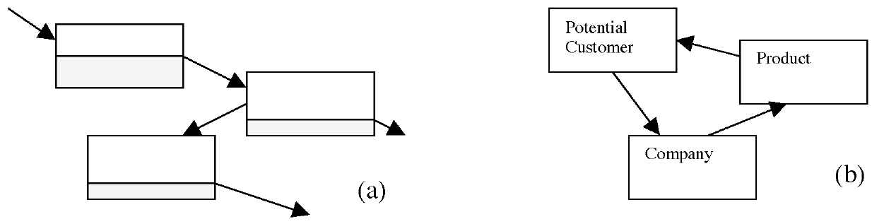
Figure 1 Comparison between a simple and a complex system
- The company produces a particular product. This results from the beliefs at which the company has arrived concerning the kind of customers that are “out there” and the qualities they are looking for at the price they are willing to pay. The arrow therefore encompasses the way in which the marketing people in the company have been able to affect the designer and the new product development process to try to produce the “right thing at the right price.” Secondly, it implies that the designer knows how to put components together in such a way that the product or service “delivers” what was hoped.
- The product then attracts, or fails to attract, potential customers. However, this requires the potential customers to “look at” the product and see what it might do for them, and at what cost. Customers must be able to translate the attributes of the product or service into the fulfillment of some need or desire that they have. The “interaction” between the product and the customer must be “engineered” by the company so that there will be some encounter with potential customers. The locations and timings must therefore be suited to the movements and attention of the potential target customers.
- The arrow from the customer to the company finally consists of a flow of money that occurs when a potential customer becomes an actual customer. This part is physical and real and can be stored easily on a database. However, it is the “result” of a whole lot of less palpable processes, of conjecture, of characterization, and of information analysis, most of which do not correspond to flows of anything accountable.
What is important is that inside each “box” there are multiple possible behaviors. Ultimately, this comes down to the existence of internal microdiversity that gives each box a range of possible responses. These are tried out and the results used either to reinforce or to challenge their use. Each box is therefore trying to make sense of its environment, which includes the other boxes and their behaviors.
The real issue is that the boxes marked “company” and “potential customer” actually enclose different worlds. The dimensions, goals, aims, and experiences in these boxes are quite different. Most importantly, each box contains a whole range of possible behaviors and beliefs, and the agents “inside” may have mechanisms that enable them to find out which ones work in the environment. What this means is dealt with in the next section. When the boxes interact, therefore, as reflected in some simple “arrows” of influence, what we really have is the communication of two different worlds that inhabit different sets of dimensions. However, to “successfully” connect two different “boxes” so as to achieve some joint task requiring cooperation demands some human intervention to “translate” the meaning that exists in one space into the language and meaning of the other.
The simple “arrow” of connection, therefore, will not be a “simple connection,” but instead may require a person who is capable of speaking across the boxes and who possibly has experience of both worlds. It is also the core reason explaining the need for interdisciplinary studies. Each discipline takes a partial and particular view of a situation, and in so doing promotes analysis and expertise at the expense of the ability of integration, synthesis, and a holistic view. Management is a domain in which a multidisciplinary, integrative approach is required if we are to get real results in dealing with a real-world problem. The science of complex systems is extremely important for management and for policy, since only with an integrated, multidimensional approach will advice be related successfully to the real-world situation. This may indeed spell the limits to knowledge and turn us from the attractive but misleading mirage of prediction.
STRUCTURAL ATTRACTORS
If we consider the use of the word “attractor” in nonlinear dynamics, its meaning is associated with the long-term destination of system trajectories. These can either end at a steady final value—a point attractor—or in stationary cyclic or chaotic motion. The attractor in which the system trajectory ends up will depend on the “richness” of the possible behaviors generated by the particular nonlinear equations, and the point from which the system starts. So, we may have a situation as shown in Figure 2, where there are several attractors of different types, and the equations drive the system toward the long-term stationary attractor of the “basin of attraction” in which it starts.

Figure 2 An imaginary view of the possible attractors of a particular set of nonlinear equations. All the attractors correspond to stationary, cyclic, or chaotic values of x and y . These are not “structural attractors.”
In fact, these attractors correspond to the end states of a given dynamic. The variables in play are fixed and do not change. Only their values change and so the “dimensionality” of the system remains constant. However, in Table 1 we see that this corresponds only to systems that can legitimately be described by a set of dynamical equations describing the changes over time in the values of a given set of variables. Even if we consider self-organizing systems that have probabilistic rates of interactions, the noise can simply push the system over the boundaries separating attractor basins, leading to changes in the configuration and behavioral regime of the given set of variables. Even then, the only dimensional changes that can occur are those associated with the emergent properties of the whole system. The “internal dimensions” of the interacting variables are not changed.
What happens if we consider the evolution of a system that has different types of individual interacting—different subjectivities—with different dimensions and attributes. We may say that if all the possible types were present simultaneously, we would have an enormously diverse system with a vast range of attributes and dimensions present. However, evolution results in a selection process that reduces the types of individual or agent that can inhabit the system to those that can coexist with or have synergy with the other types present.
For this simple model, we consider the interaction of populations of agents with different attributes and behaviors, which may affect, positively or negatively, the populations with which they cohabit. This leads to a model in which the “payoffs” that are found for the behavior exhibited by a particular population type depend on the other behaviors present in the system. Instead of the problem being one in which the evolutionary task is to explore and climb a fixed landscape of “fitness” or “payoff,” the landscape itself is changed by the presence of the different players in the game.
In order to examine how populations may evolve over time, let us consider 20 possible populations, agent types, or behaviors. In the space of “possibilities,” numbered 1 to 20, closely similar behaviors are considered to be most in competition with each other, since they occupy a similar niche in the system. Any two particular populations, i and j, may have an effect on each other. This could be positive, in that side effects of the activity of j might in fact provide conditions or effects that help i. Of course, the effect might equally well be antagonistic, or neutral. Similarly, i may have a positive, negative, or neutral effect on j. For our simple model, therefore, we shall choose values randomly for all the possible interactions between all i and j; fr describes the average strength of these, and 2*(rnd − 0 .5) is a random number between -1 and +1.
Interaction(i, j) = fr * 2 * (rnd − 0.5)
The effect of behavior i on j will be proportional to the size of the population i. If i is absent, there will be no effect. Similarly, if j is absent, it cannot feel the effect of i. For each of 20 possible types we choose the possible effect i on j and j on i randomly, where random(j,i) is a random number between 0 and 1, and fr is the strength of the interaction. Clearly, on average we shall have equal numbers of positive and negative interactions.
Each population that is present will experience the net effect that results from all of the other populations that are also present. Similarly, it will affect those populations by its presence.
Net Effect on i = Σ jx(j).Interaction(j,i)
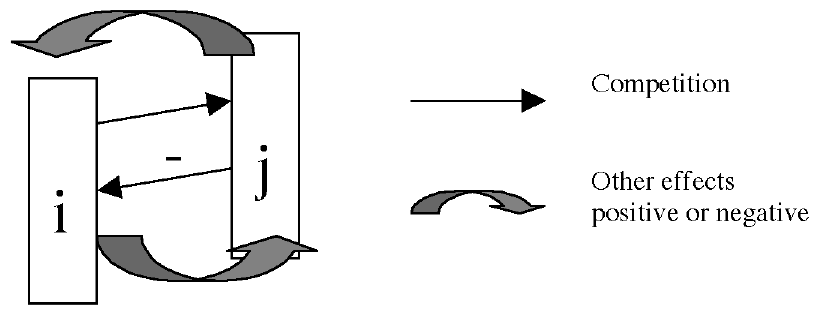
Figure 3 Each pair of possible behaviors, types i and j, has several possible effects on each other. First, they compete for resources. But secondly, each one may have effects that are either antagonistic, neutral, or synergetic on the other.
The sum is over j including i, and so we are looking at behaviors that in addition to interacting with each other also feed back on themselves. There will also always be a competition for underlying resources, which we shall represent by:
At any time, then, we can draw the landscape of synergy and antagonism that is generated and experienced by the populations present in the system. We can therefore write down the equation for the change in population of each of the xi It will contain the positive and negative effects of the influence of the other populations present, as well as the competition for resources that will always be a factor, and also the error-making diffusion through which populations from i create small numbers of offspring in i + 1 and i - 1.
where f is the fidelity of reproduction. The first group of terms corresponds to growth of x(i), due to natural growth, and as inward diffusion from the populations of type x - 1 and x + 1. The growth rate reflects the “net effects” (synergy and antagonism) on x(i) of the presence of populations other than x(i). There are limited resources (N) available for any given behavior, so it cannot grow infinitely. The final term merely reflects the natural lifetime of any active x.
Let us consider a typical simulation that this model produces. If we start initially with a single population present, for example x(11) = 5 and all other populations are 0. If we plot the net effect of this population on the other 19 possible populations it will provide a simple onedimensional “landscape” showing the potential synergy/antagonism that would affect each population if it were to appear. The only population initially present is x(11) and therefore the evolutionary landscape in which it sits is in fact that which it creates itself. No other populations are yet present to contribute to the overall landscape of mutual interaction.
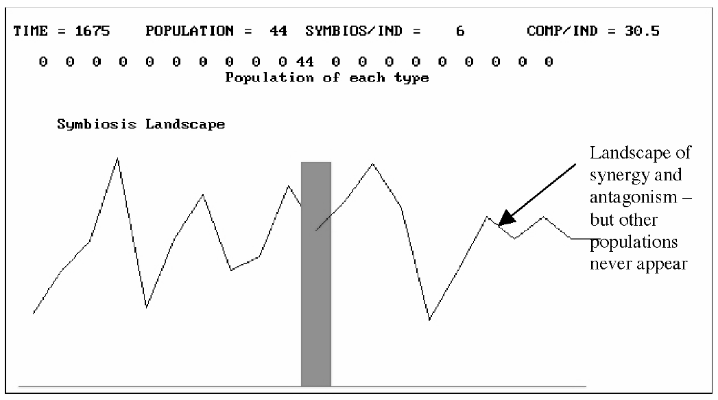
Figure 4 With no exploration in character space, fidelity f = 1, the system remains homogeneous, but its performance will only support a population of 44.
The system rapidly reaches a steady state with the low population of 44. The competition per individual is over 30 units and symbiosis per individual is only 6.
If the same simulation is repeated with the same hidden pair interactions and the same initial conditions, but this time there is a 2 percent “exploration” from any population into the adjacent character cells, then the result is as shown in Figure 5 and 6 overleaf. We see that the performance of the system increases to support a population of 72, the competition experienced per individual falls to 19, and the symbiosis per individual rises to 26.
What matters, then, is how the population 11 affects itself. This may have positive or negative effects depending on the random selection made at the start of the simulation. However, in general the population 11 will grow and begin to “diffuse” into the types 10 and 12. Gradually, the landscape will reflect the effects that 10, 11, and 12 have on each other, and the diffusion will continue into the other possible populations. Hills in the landscape will be climbed by the populations, but as they climb they change their behavior and therefore change the landscape for themselves and the others. Figures 5 and 6 show this process taking place over time.
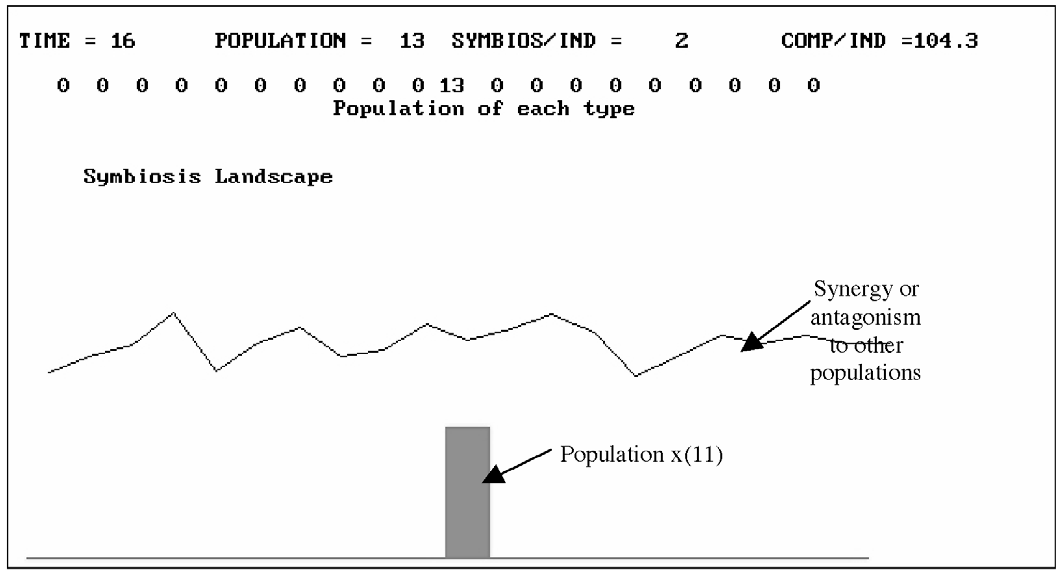
Figure 5 The initial population and evolutionary landscape of our simulation (Time 16).
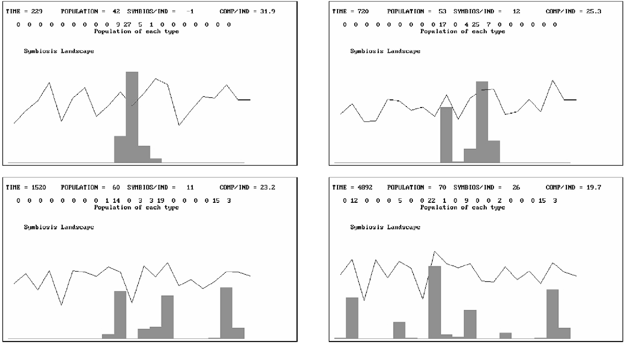
Figure 6 The sequence of events (times 229, 720, 1520, and 4892) that lead to a structural attractor involving populations 2, 6, 9, 12, 15, 19, and 20.
However, we can ask whether this “structural attractor” involving the reduced dimensions and attributes associated with the populations that coexist in the attractor is the only one possible for a given set of potential interactions between i and j. The answer is no. There are several attractors possible and they involve different populations, and different dimensions and attributes. They are qualitatively different from the first attractor. For example, in Figure 7 we see a stable structure that results when the same system as before is started from x(1) instead of x(11).
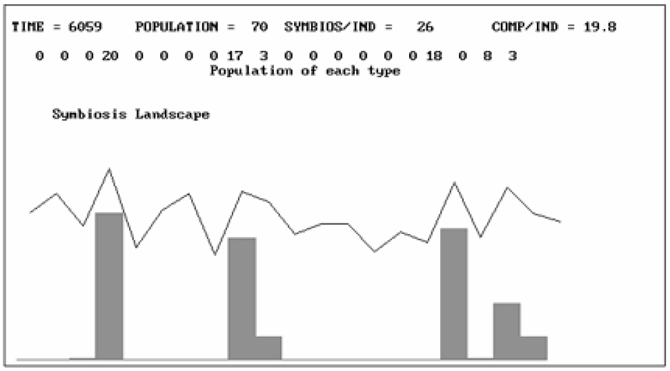
Figure 7 An alternative outcome for identical pair interactions, but for an initial seed placed at population 1 instead of 11. This involves 4, 9, 10, 17, 19, and 20.
Clearly, this shows us that the dynamics are path dependent and so, even with the same potential interactions, qualitatively different situations can emerge. Obviously, if we choose a different set of pair interactions to “explore” with our model, we shall find different attractors.
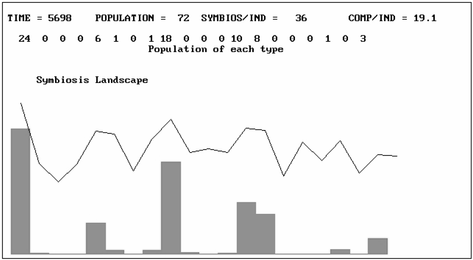
Figure 8 If there are different pair interactions between potential populations, the model generates a different set of attractors.
IMPLICATIONS: WHAT IS A COMPLEX SYSTEM?
There are several important points about these results. The first is that they are generic and the results apply very generally. If we cannot make assumptions 3 and 4 mentioned in the introduction (average behavior, smooth processes), which take out the microdiversity and idiosyncracy of real life agents, actors, and objects, we automatically obtain the emergence of a structural attractor. This is a complex system of interdependent behaviors whose attributes are on the whole synergetic. These have better performance than their homogeneous ancestors, but are less diverse than if all “possible” behaviors were present. They correspond to the emergence of hypercycles in the work of Eigen and Schuster (1979). Those present result from the particular history of search undertaken, and on their synergy. In other words, a structural attractor is the emergence of a set of interacting factors that have mutually supportive, complementary attributes.
What are the implications of these structural attractors?
- Search carried out by the “error-making” diffusion in character space leads to vastly increased performance of the final object. Instead of a homogeneous system, characterized by intense internal competition and low symbiosis, the development of the system leads to much higher performance, and one that decreases internal competition and increases synergy.
- The whole process leads to the evolution of a complex, a “community” of agents whose activities, whatever they are, have effects that feed back positively on themselves and the others present. It is an emergent “team” or “community” in which positive interactions are greater than the negative ones.
- The diversity, dimensionality, and attribute space occupied by the final complex are much greater than the initial homogeneous starting structure of a single population. However, they are much less than the diversity, dimensionality, and attribute spaces that all possible populations would have brought to the system. The structural attractor therefore represents a reduced set of activities from all those possible in principle. It reflects the “discovery” of a subset of agents whose attributes and dimensions have properties that provide positive feedback. This is different from a classical dynamic attractor that refers to the long-term trajectory traced by the given set of variables. Here, our structural attractor concerns the emergence of variables, dimensions, and attribute sets that not only coexist but actually are synergetic.
- A successful and sustainable evolutionary system will clearly be one in which there are freedom and encouragement for the exploratory search process in behavior space. The system can generate a fairly stable community of agents or actors by having the freedom to explore. Also, the self-organization of our system leads to a highly cooperative system, where the competition per individual is low, but where loops of positive feedback and synergy are high. In other words, the free evolution of the different populations, each seeking its own growth, leads to a system that is more cooperative than competitive. The vision of a modern, free-market economy leading to, and requiring, a cut-throat society where selfish competitivity dominates, is shown to be false, at least in this simple case.
The most important point is the generality of the model presented above. The model concerns the exploration of possible behaviors by agents, each with their own characteristics and dimensions, and a selection process that retains the successful experiments and suppresses the unsuccessful. Clearly, this situation characterizes almost any group of humans: families, companies, communities, etc., but only if the exploratory learning is permitted will the evolutionary emergence of structural attractors be possible. If we think of an artifact, some product resulting from a design process, then there is also a parallel with the emergent structural attractor. A product is created by bringing together different components in such a way as to generate some overall performance. But, there are several dimensions to this performance, concerning different attributes. These, however, are correlated so that a change that is made in the design of one component will have consequences for the performance in different attribute spaces. Some may be made better and some worse.
Our emergent structural attractor is therefore relevant to understanding what successful products are and how they are obtained. Clearly, a successful product is one that has attributes that are in synergy, and that lead to a high average performance. From all the possible designs and modifications, we seek a structural attractor that has dimensions and attributes that work well together. This is arrived at by R&D that must imitate the exploratory search of possible modifications and concepts that is “schematically represented” by our simple model above. A successful design for an automobile, aircraft, or even a simple wine glass will be a “structural attractor” within the space of possible designs, techniques, and choices that have emerged through a search process.
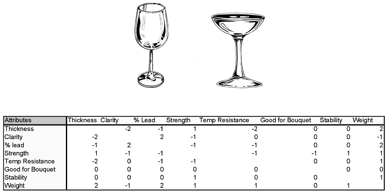
Figure 9 Imaginary pair-wise attribute interaction table for a “wine glass.” This would replace our “random” assignment in the general model above.
This shows us that although a “wineglass” is not itself a complex system, it is produced by a complex system. The complex system searches and discovers what combinations of shape, thickness, glass composition, etc. lead to attributes that are mutually compatible and desired. Part of the complex system that produces the wine glass is about the technology and production processes that lead to the attributes of the emergent objects. This is why the organizational forms, the technologies, and the skill bases that underlie wine glasses over time will in fact evolve through successive stages, just like our simple model above.
However, although our model shows us how the presence of exploration in character space will lead to emergent objects and systems with improved performance, it is still true that we cannot predict what they will be. Mathematically, we could solve our equations to find the values of the variables for an optimal performance. But, we do not know which variables will be present, and therefore we do not know which equations to solve or optimize. In our model we used random numbers to choose pair-wise interactions in an unbiased way, but in fact in a real problem these are not “random” but reflect the underlying physical, psychological, and behavioral reality of the processes and components in question. By considering the underlying reality, we could estimate these values for each pair and then see what kind of structural attractors our simulation might produce. This would lead to a “cladistic diagram” (a diagram showing evolutionary history), suggesting how a system had changed and evolved structurally over time. It would generate an evolutionary history of both artifacts and the organizational forms that underlie their production (McKelvey, 1982, 1994; McCarthy, 1995; McCarthy, Leseure, Ridgeway, and Fieller, 1997).
Another important point, particularly for scientists, is that it would be extremely difficult to discern the “correct” model equations, even for our simple 20-population problem, from observing the population dynamics of the system. Because any single behavior could be playing a positive or negative role in a self, or pair or triplet etc., interaction, it would be impossible to “untangle” its interactions and write down its equations simply by noting the population's growth or decline. Despite the difficulty of an “observing scientist” predicting the structural attractor, the system itself can generate one quite easily. All it needs is to have the microdiversity of its error-making search process running, and it will find stable arrangements of multiple actors. It will discover a balance between the agents in play and the interactions that they bring with them. But, although the system can do this automatically, it does not mean that we can know what the web of interactions really is.
This certainly poses problems for the rational analysis of situations, since this must rely on an understanding of the consequences of the different interactions that are believed to be present. We cannot really know from the decontextualized data of growth and decline how the circles of influence really operate. Our only choice might be to ask the actors involved, in the case of a human system. And this, in turn, would raise the question of whether people really understand the foundations that sustain their own situation, and the influences of the functional, emotional, and historical links that build, maintain, and cast down organizations and institutions. The loops of positive feedback that build structure introduce a truly collective aspect to any profound understanding of their nature, and this will be beyond any simple rational analysis, used in a goal-seeking, local context.
CONCLUSION
The science of complex systems is about systems whose internal structure is not reducible to a mechanical system. In particular, it is about connected complex systems, for which the assumptions of average types and average interactions are not appropriate and are not made. Such systems coevolve with their environment, being “open” to flows of energy, matter, and information across whatever boundaries we have chosen to define. These flows do not obey simple, fixed laws, but instead result from the internal “sense making” going on inside them, as experience, conjectures, and experiments are used to modify the interpretive frameworks within. Because of this, the behavior of the systems with which each system is coevolving are necessarily uncertain and creative, and is not best represented by some predictable, fixed trajectory. This takes some steps toward the “postmodern” point of view. But, as Cilliers (1998) indicates, the original definition of postmodernism (Lyotard, 1984) does not take us to the situation of total subjectivity where no assumptions can be made, but rather to the domain of evolutionary complex systems discussed in this article.
Instead of a fixed landscape of attractors, and a system operating in one of them, we have a changing system, moving in a changing landscape of potential attractors. Provided that there is an underlying potential of diversity, then creativity and noise (supposing that they are different) provide a constant exploration of “other” possibilities. Our simple model only supposed 20 possible underlying behaviors, but obviously in any realistic human situation the number would be very large. In dealing with a changing environment, therefore, we find a “law of excess diversity” in which system survival in the long term requires more underlying diversity than would be considered requisite at any time. Some of these possible behaviors mark the system and alter the dimensions of its attributes, leading to new attractors and new behaviors, toward which the system may begin to move but at which it may never arrive, as new changes may occur “on the way.” The real revolution is not therefore about a neoclassical, equilibrium view as opposed to nonlinear dynamics having cyclic and chaotic attractors, but instead is about the representation of the world as a nonstationary situation of permanent adaptation and change. The picture we have arrived at here is one that Stacey et al. (2000) refer to as a “transformational teleology,” in which potential futures (patterns of attractors and of pathways) are being transformed in the present. The landscape of attractors we may calculate now is not in fact where we shall go, because it is itself being transformed by our present experiences.
The macro-structures that emerge spontaneously in complex systems constrain the choices of individuals and fashion their experience. Behaviors are being affected by “knowledge” and this is driven by the learning experience of individuals. Each actor is coevolving with the structures resulting from the behavior and knowledge/ignorance of all the others, and surprise and uncertainty are part of the result. The “selection” process results from the success or failure of different behaviors and strategies in the competitive and cooperative dynamical game that is running.
However, there is no single optimal strategy. What emerge are structural attractors, ecologies of behaviors, beliefs, and strategies, clustered in a mutually consistent way, and characterized by a mixture of competition and symbiosis. This nested hierarchy of structure is the result of evolution and is not necessarily “optimal” in any way, because there is a multiplicity of subjectivities and intentions, fed by a web of imperfect information and diverse interpretive frameworks. In human systems, at the microscopic level, behavior reflects the different beliefs of individuals based on past experience, and it is the interaction of these behaviors that actually creates the future. In so doing, it will often fail to fulfill the expectations of many of the actors, leading them either to modify their (mis)understanding of the world, or alternatively simply leave them perplexed. Evolution in human systems is therefore a continual, imperfect learning process, spurred by the difference between expectation and experience, but rarely providing enough information for a complete understanding.
Although this sounds tragic, it is in fact our salvation. It is this very “ignorance” or multiple misunderstandings that generates microdiversity, and leads therefore to exploration and (imperfect) learning. In turn, the changes in behavior that are the external sign of that “learning” induce fresh uncertainties in the behavior of the system, and therefore new ignorance (Allen, 1993). Knowledge, once acted on, begins to lose its value. This offers a much more realistic picture of the complex game that is being played in the world, and one that our models can begin to quantify and explore.
In a world of change, which is the reality of existence, what we need is knowledge about the process of learning. From evolutionary complex systems thinking, we find models that can help reveal the mechanisms of adaptation and learning, and that can also help imagine and explore possible avenues of adaptation and response. These models have a different aim from those used operationally in many domains. Instead of being detailed descriptions of existing systems, they are more concerned with exploring possible futures and the qualitative nature of these. They are also more concerned with the mechanisms that provide such systems with the capacity to explore, to evaluate, and to transform themselves over time. They address the “what might be,” rather than the “what is” or “what will be.” It is the entry into the social sciences of the philosophical revolution that Prigogine wrote about in physics some 25 years ago. It is the transition in our thinking from “Being to Becoming.” It is about moving from the study of existing physical objects using repeatable objective experiments, to methods with which to imagine possible futures and with which to understand how possible futures can be imagined. It is about system transformation through multiple subjective experiences, and their accompanying diversity of interpretive, meaning-giving frameworks.
Reality changes, and with it experiences change also. In addition, however, the interpretive frameworks or models people use change, and what people learn from their changed experiences is transformed. Recognizing these new “limits to knowledge,” therefore, should not depress us. Instead, we should understand that this is what makes life interesting, and what life is, has always been, and will always be about.
ACKNOWLEDGMENTS
This work was partially carried out under the EPSRC Nexsus Network program. The idea of “structural attractors” occurred during a discussion with J. McGlade and M. Strathern.
References
Allen, P M. (1988) “Evolution: Why the whole is greater than the sum of its parts,” in W . Wolff, C.-J. Soeder, & F R. Drepper (eds) Ecodynamics, Berlin, Germany: Springer.
Allen, P M. (1990) “Why the future is not what it was,” Futures, July/August: 555-69.
Allen, P M. (1993) “Evolution: Persistent ignorance from continual learning,” in Nonlinear Dynamics and Evolutionary Economics, Oxford, UK: Oxford University Press: 101-12.
Allen, P M. (1994a) “Coherence, chaos and evolution in the social context,” Futures, 26(6): 583-97.
Allen, P M. (1994b) “Evolutionary complex systems: Models of technology change,” in L. Leydesdorff & P van den Besselaar (eds), Chaos and Economic Theory, London: Pinter.
Allen, P M. (2000) “Knowledge, learning, and ignorance,” Emergence, 2(4): 78-103.
Allen, P M. & McGlade, J. M. (1987) “Evolutionary drive: The effect of microscopic diversity, error making and noise,” Foundations of Physics, 17(7, July): 723-8.
Cilliers, P (1998) Complexity and Post-Modernism, London and New York: Routledge.
Eigen, M. & Schuster, P (1979) The Hypercycle, Berlin, Germany: Springer.
Lyotard, J.-F (1984) The Post-Modern Condition: A Report on Knowledge, Manchester, UK: Manchester University Press.
McCarthy, I. (1995) “Manufacturing classifications: Lessons from organisational systematics and biological taxonomy,” Journal of Manufacturing and Technology Management— Integrated Manufacturing Systems, 6(6): 37-49.
McCarthy, I., Leseure, M., Ridgeway, K. & Fieller, N. (1997) “Building a manufacturing cladogram,” International Journal of Technology Management, 13(3): 2269-96.
McKelvey, B. (1982) Organizational Systematics, San Francisco: University of California Press.
McKelvey, B. (1994) “Evolution and organizational science,” in J. Baum & J. Singh, Evolutionary Dynamics of Organizations, Oxford, UK: Oxford University Press: 314-26.
Stacey, R., Griffen, D., & Shaw, P. (2000) Complexity and Management, London and New York: Routledge.