Introduction
Extensive studies of innovation diffusion have shown that it obeys a logistic equation, so far. The innovation paradigm has a latent period of technological development before product diffusion. We have studied this technological development period and succeeded in describing the comprehensive paradigm of innovation with nonlinear logistic trajectories (Hirooka, 1999, 2001, 2003a,b, 2005b). We (Hirooka, 1994, 2002, 2003b,c, 2004a, 2005a) also found that the diffusion of innovations gathers along the upswing of a Kondratiev business cycle. The present study was carried out on the basis of these analyses, which indicate that innovation systems have a logistic nonlinear nature.
The innovation system is discrete and dissipative; it is created by knowledge transfer from person to person as a steadily changing nonlinear stream. Griliches (1957) first pointed out, and many economists have confirmed, that the diffusion of innovations has a logistic nature, meaning that the system is nonlinear. On the other hand, the epoch-making analysis by May (1974, 1976) revealed deterministic chaos in logistic mapping. May found the bifurcation phenomenon in the ergodic region in which multiple solutions with a periodicity are obtained. Peters (1991) pointed out that, even in the chaotic region, there is a window of chaos in which there is a regular iterative structure and existence of a specific order. From this trend, he argued that the logistic mapping has a fractal nature. Goodwin (1950, 1982, 1990, 1991) analyzed Schumpeter’s concept of complex business cycles, which are Kondratiev cycles combined with Juglar cycles, using a logistic difference equation and clarified the nature of the chaotic dynamics. Lorenz (1993) summarized his ‘nonlinear economics’ which encompasses chaotic dynamics, bifurcation theory, Goodwin’s model, class struggle model based on the Lotka-Volterra equation, and logistic complex systems.
Peters (1991) defined nonlinear dynamic systems as systems that have:
The feedback system means that a previous event affects a next event as described in the mapping of the logistic equation. The critical level that produces at least two equilibriums indicates the region in which the bifurcation phenomenon occurs: in the case of May’s logistic mapping, it is the region of a > 2.5 (seems to be > 3). All of these analyses focused on the discrete logistic equation and indicate that innovation should be discussed in this context. However, there has been no empirical analysis using concrete data on innovation. This paper is a trial to study the complexity in innovation systems based on empirical analysis and examines the nature of logistic complexity in a mathematical context.
Structure of innovation systems
The present analysis is based on the methodology we have developed for analyzing innovation systems by using three trajectories. This analysis first started from the fact that innovation diffusion obeys a logistic equation.
Description of innovation diffusion
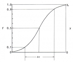
Since the first Industrial Revolution, the economy has developed through innovations creating economic infrastructures. The diffusion of innovations can be described by a logistic equation, as first pointed out by Griliches (1957), and many economists have confirmed this. Some authors, however, have proposed alternative or modified models for describing the diffusion of innovations. Because the diffusion of new products in the market is quite often retarded by various types of economic turbulence, such as recession and war, evaluating whether the equation fits the diffusion profile well is rather difficult. Previous research (Hirooka & Hagiwara, 1992; Hirooka, 1995, 2003a,b,c, 2004a, 2005a,b) demonstrated that the diffusion of innovation products proceeds according to a logistic equation in a sound economy but is disturbed by economic turbulence. This is clarified when diffusion is analyzed using a Fisher-Pry plot which makes a straight line. The logistic equation and its derivation to Fisher Pry plot are described in Appendix 1. The actual S curve of logistic equation with a time span of ?t is illustrated in Figure 1.
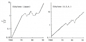
The diffusion process was examined using the above procedure with Fisher Pry plot for 17 products, including five bulk chemicals, four engineering plastics, six electric appliances, crude steel, and automobiles (Hirooka & Hagiwara, 1992; Hirooka, 2003c). The linear correlations of the Fisher Pry plots for the 17 products were verified and the intrinsic diffusion coefficient ‘a’ was determined based on the flex point. The coefficients are shown in Table 1 together with the time spans. ‘Intrinsic’ means the coefficients were calculated by determining the slopes of the Fisher Pry plots, excluding the delay caused by economic turbulence. Typical examples of Fisher Pry plot are shown in Figure 2 in the case of ethylene production in Japan and the US.
Logistic?equation?and?time?span??t
These results clearly indicate that:
The diffusion of new products obeys a simple logistic equation during sound economic periods;
The diffusion is easily disturbed by economic turbulence, such as recession and war, so that the demand for products greatly decreases, diverging from the original locus;
It is noteworthy that after a recession, the diffusion of the products resumes, taking the same slope of Fisher Pry plot as before the recession. This strongly supports that the diffusion of a product has an inherent trajectory with an intrinsic diffusion coefficient.
The diffusion coefficients of the products listed in Table 1 ranged between 0.23 and 0.94, and the time spans were between 4.5 and 19.0 years.
Estimation of technological development period and comprehensive description of innovation paradigm
An innovation paradigm consists of two periods: technological development and product diffusion in that order. While the innovation diffusion period lasts for about 25 to 30 years until the market matures, the technological development period lasts for about the same number of years before starting the product diffusion period. The economics of technological change has mostly addressed the diffusion period.
Logistic?diffusion?of?ethyl?ene?in?Japan?and?the?United?States
Source: Hirooka & Hagiwara, 1992; Hirooka, 2003c.
Table?1
Diffusion coefficients of innovation products for the Japanese market (source: Hirooka & Hagiwara, 1992; Hirooka, 2003c)
The technological development period has not been so extensively studied so far. Marchetti (1979: 80) disclosed that various technologies developed in accordance with a logistic equation and Andersen (2001) revealed that the development of patents in various technological fields can be described by a logistic equation. Hirooka (2003a,b) confirmed the logistic nature of innovation as well, and further established a method of how to determine the logistic development profile. That is, as far as the technological development period in an innovation can be described by a logistic equation, the various elements during the course of innovation should be substantially distributed within a definite time span of ?t. When the time span is measured from the distribution of innovation elements over time, the logistic trajectory is apriori determined only by the time span. As the innovation process is a discrete phenomenon, this procedure is sufficiently applicable to a surge of innovation elements. This procedure was successfully applied to determine various innovation profiles. We have devoted ourselves to analyzing the technological development period in depth and have clarified various interesting features (Hirooka & Hagiwara, 1992, Hirooka, 1994, 1995, 1999, 2001, 2002, 2003a, b, c, 2005b).
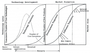
Through such analyses, we found that the technological development period comprises two trajectories: technology and development ones. The first one starts with the initial basic invention or epoch-making discovery, and various core technologies form a cluster that comprises the technology trajectory. A series of innovation products are then developed that comprise the development trajectory.
It is interesting to note that the diffusion trajectory starts just after the technology trajectory has completed, making a kind of cascade structure. These relationships are schematically shown in Figure 3. The first basic patent will often be granted during the technology trajectory. While the core technologies accumulate, new products begin to be developed using them during the last part of the technology trajectory. Commercialization begins several years later, which is the beginning of the diffusion trajectory. After the introduction period, which has a rather slow pace, business quickly picks up, and many newcomers enter the market, inducing in what Schumpeter called the “bandwagon effect.” Determination of the trajectories is described in Hirooka (2003a, 2005b).
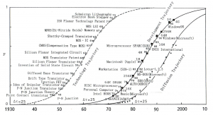
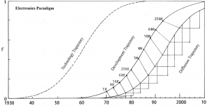
For the electronics innovation paradigm, the interrelations between the three trajectories are illustrated in Figure 4. The technology trajectory started with the epochal invention of the transistor by Shockley, et al. in 1948. It was carried forward by various core inventions: solid state circuits by Kilby, monolithic integrated circuits by Noyce, and MOS (metal-oxide-semiconductor) integrated circuits. It ended with the completion of submicron lithography technology by IBM in 1973. The development trajectory comprises a series of IC products developed in accordance with Moore’s law and has a time span of 25 years. The diffusion trajectory is the history of demand for IC chips, as shown by the black dots in Figure 4.
Fractals in electronics paradigm
It is revealed that innovation paradigms comprise various fractals, and these fractals are essential elements because each trajectory is formed by the accumulation of discrete phenomena, which are small structural elements. There are two types of fractals: chain and bundle. The first type form in a series, a chain structure, along the trajectory as its constituents. The second type form like a bouquet of flowers, a bundle structure, along the trajectory.
Structure?of?innovation?paradigm?with?three?trajectories
Innovation?paradigm?of?electronics
Source: Hirooka, 2003a.
Chain fractals of IC devices
Regarding the development of innovation technologies, the development technology consists of a series of developments of innovation products. Each innovation product is distinct and has its own development history with a shorter development trajectory. This is the origin of fractals. For instance, devices in the electronics paradigm are developed step by step, following Moore’s law. That is, the degree of device integration quadruples every three to four years from one grade to the upper grade. The development is not continuous but a stepwise process. Each process has its own trajectory that is an element of the fractal, and the accumulated fractals compose the parent development trajectory. The resulting products diffuse, forming a diffusion trajectory with a chain fractal structure, as shown in Figure 5. The transition of developments of integrated circuits is located on the development trajectory; a few years later, the developed product is sold along the diffusion trajectory. The sale of an IC chip continues for several years until it is replaced by a more advanced one. This process is described by a triangle on the diffusion trajectory, as shown in Figure 5. The fractals form a chain structure.
Bundle fractals in application fields
Another fractal structure can be seen in the application fields. The development trajectory comprises various developed products and also various applications. The development history of innovation products composes the development trajectory, and the products diffuse to be used in various applications, forming a fusion trajectory, as described in previous research (Hirooka, 1999, 2003a, 2005b). The adoption of innovation by existing industries was termed ‘technology fusion’ by Kodama (1985) and Freeman (1987). Thus, a trajectory based on technology fusion is called a ‘fusion trajectory’. This means that an innovation expands beyond its own products towards wider application through the techno-economic paradigm change. For example, the electronics devices not only form an electronics development trajectory, they were also adopted by various industries for use in a wide variety of products, including aircraft engines, machine tools, automobiles, and cameras. Each industry creates its own fusion trajectory, as discussed in Hirooka (1999, 2003a, 2005b). These fusion trajectories occur along the electronics development trajectory, meaning that the adoption of electronics innovations by other industries takes place at the same time as the original product development. The time span of these fractal trajectories is almost the same as that of the original development trajectory because the development of technology fusion takes place along the development trajectory. These fractals form a bundle of fusion trajectories along the electronics development trajectory, as shown in Figure 6. It is amazing to see how quickly other industries adopt innovation technologies. This expanded use of innovation technologies enriches the development trajectory and expands the market, contributing to institutional change in the economy.
Fractal?structure?of?IC?chips?in?electronics?paradigm
Source: data in Japanese market by MITI statistics.
Fractals?of?fusion?trajectories?of?various?industries?in?electronics?paradigm
Source: Hirooka, 1999c, 2003a.
System fractals in innovation paradigms
Evolution of information technology paradigms
The information technologies are summarized into three paradigms: computers, electronics, and multimedia. While these are different paradigms established within individual disciplines, they closely interact and together form the modern information society. The computer system has evolved by adopting electronics, and the multimedia system has been constructed on the basis of computer and electronics technologies. The evolutionary trend of these three paradigms can be illustrated in Figure 7, by using two loci: the development and diffusion trajectories. The relative positioning of these trajectories indicates that the computer and electronics paradigms are mature while the multimedia one is still premature. This gap provides an important insight into the IT recession. There was a bubble phenomenon in the electronics and information businesses around 2000, and the economy then entered a kind of air pocket: IT recession. According to Perez’s (2002) explanation, we are now at a turning point, from a ‘frenzy’ phase to a ‘synergy’ phase. Since the multimedia paradigm is still not mature enough to add sufficient value to the economy, the economy cannot yet enjoy the fruits of multimedia. This gap is one explanation for the present slackness in the economy. The synergy phase should take effect during the upswing of the 5th Kondratiev wave towards the peak of 2040. The electronics and information infra-trajectory will enter the second full-swing phase, as described in Hirooka (2004a).
Evolution?of?information?technology?paradigms?and?fractals
Source: Hirooka & Nitta, 2002; Hirooka, 2003a, 2004b.
Fractals of technological systems
After the completion of the core technologies composing the technology trajectory, a series of new products are developed composing the development trajectory. Furthermore, various elementary technological systems are developed along the development trajectory using the core technologies. These systems are intermittently invented to support the development of new products or as applications of these products. These are more sophisticated and complex systems, than simple products directly prepared using core technologies. They sometimes comprise combinations with some devices and software.
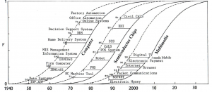
The development trend of various elementary technological systems is illustrated by bars on the development trajectory in Figure 7. The starting point of each bar indicates the timing of the invention of the technological system, and the end of the bar corresponds to the practical use of the system along the stream of the diffusion trajectory, but this last point does not always correspond to the timing of commercialization. Each bar can be substantially considered to correspond to a small fractal S-curve because each technological system development can be expressed using a small logistic curve. That is, the development trajectory also functions as a locus of an accumulated cluster of relevant elementary technological systems.
In the computer paradigm, computers were first used for scientific and military purposes. They were later (around 1960) put to use for business purposes (accounting, etc.). The package home delivery system in Japan began using computers in 1968. Information management and decision support systems were developed in around 1970. Office automation systems came into use in 1974, and then factory automation systems became operable. This is the trend of elementary technological systems using computers.
The development of microprocessors in 1971 initiated the electronics development trajectory. Machine tools were first equipped with microprocessors for numerical control. This led to the development of FMS (flexible manufacturing systems) comprising computer controlled machine tools, robots, and unmanned carriers. POS (Point of Sales) systems were developed in 1983 and soon became widely used in retail businesses. The CALS (Computer-Aided Acquisition and Logistics Support) system was developed as a computer-aided procurement system by the U.S. Department of Defense in 1985. At the same time, strategic information systems (SIS) were adopted by leading firms for comprehensive management of their entire business. Various industries began developing civil use CALS (Commerce At Light Speed) systems in 1994.
The age of multimedia began with the Internet system, originally known as NSFNET, in 1990. Now that we are in the multimedia paradigm, electronic commerce has begun to take shape, and electronic money has been commercialized. An important symbol of multimedia was the start of digital television broadcasting in the UK and US in 1998. These chain fractals of elementary technological systems compose the multimedia paradigm.
Other fractals in innovation systems
In the case of the chemical industry, many innovation products were developed, as shown in Table 1, and the development and diffusion trajectories of the polymer industry paradigm, which both have a time span of 35 years, are composed of these fractals.
In general, the development and diffusion trajectories are composed of an assortment of various chain and bundle fractals. Furthermore, Hirooka (2004a) has identified a cluster of infra-trajectories across two Kondratiev cycles as an extension of the innovation paradigm. This kind of cluster also seems to be a bundle fractal of infra-trajectories.
Schumpeter (1939) insisted the complex dynamism of three business cycles composed of Kondratiev, Juglar, and Kitchin cycles. This thought can be interpreted as a kind of fractal mechanism. As shown by the above analysis, there is no doubt that fractals compose the innovation paradigm. Table 1 interestingly indicates that the time spans of innovation products of chemicals, crude steel, and automobiles are gathered in a time period of around 10 years, ranging from 9 to 19 years, actually. This is substantially the same as the time span of a Juglar cycle. Both semiconductor integrated circuits and electric appliances each have a time span of around four years (at most less than ten), which corresponds to that of Kitchin. It can thus be said that Schumpeter implicitly recognized the existence of fractals.
Self-organization in innovation paradigms
Self-organization is an important phenomenon in dissipative structures and complex systems. The self-organization in innovation systems is examined next.
Kondratiev business cycles and innovation diffusion
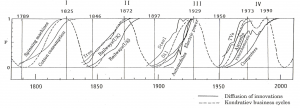
Kondratiev business cycles were identified based on the degree of economic development determined by the use of GNP and other economic aggregates. Since technological innovations add value to the economy, the level of innovation diffusion reflects the increasing value added to the new market. Therefore, the diffusion curve of innovation products is proportional to the increasing value added by the innovation per se. More importantly, the diffusion curve has a nonlinear S-shape, which means the diffusion tends to saturate within a definite time span. This makes it possible to locate the relevant innovation. We thus attempted to determine where the diffusion curves of innovation products are located on the Kondratiev cycles. The locus of the diffusion of various technological innovations was plotted on a map of the Kondratiev waves. The locus of the innovation diffusion was normalized to show the saturated market to be unity. These innovations are those played a crucial role in the formation of infrastructures in the industrialized society. As shown in Figure 8, all of the innovation S-curves selectively cluster along the upswing of the Kondratiev cycle. This cluster is a kind of bundle fractal produced by a self-organization mechanism.
Self-organization of innovations
The coincidence of innovation diffusion and an upswing described above indicates that Kondratiev business cycles are induced by the clustering of innovations. At least one of the reason for the clustering of innovations is rather simple: new products resulting from innovations are difficult to be introduced in a depressed market during a downswing, the innovations stagnate, and then simultaneously take off as the economy recovers, forming the upswing. This is a simple self-organization phenomenon. It is evidenced by the delay in full-scale diffusion of railways in the UK until the upswing of the third Kondratiev cycle, starting in around 1850, even though railways were initially introduced in 1825. Further evidence is found in the retarded diffusion of automobiles in the UK due to the Great Depression and the resumed diffusion during the upswing of the fourth Kondratiev cycle. Similar behavior was found in 17 examples described in Table 1 (Hirooka & Hagiwara, 1992; Hirooka, 1995, 2003c).
Kondratiev?business?cycles?and?diffusion?of?innovations
Source: Hirooka, 1994, 2003c.
Goodwin (1990) ascribed the cause of Kondratiev cycles to a swarm of technological innovations. He explained that a disparate group of technical innovations becomes ordered into a common upsurge by self-organization.
Three trajectories of innovation paradigm are well identified. Formation of these trajectories should be a kind of self-organized action because they are narrow and well-defined. The fractal formation of fusion trajectories along the development trajectory, illustrated in Figure 6, can also be interpreted as a kind of self-organization phenomenon.
Discrete nature and complexity in innovation systems
The above analysis surely indicates that the innovation is a typical complex system. As the innovation system is discretely developed, it should be described by a difference equation but not by a differential equation. Now, let us discuss the innovation system in terms of mathematical description of logistic dynamics.
May’s logistic mapping and fractal formation
The mapping of the logistic equation has been discussed in various ways. May’s mapping in particular has received much attention because he was the first to identify deterministic chaos. May (1976) precisely analyzed logistic mapping and the details are described in Appendix 2. We have discussed the correlation of actual rate coefficients of various diffusion data as shown in Table 1 with May’s mapping and suggested that actual data are not in chaotic or ergodic regions.
An important issue is the emergence of fractals in the course of an innovation paradigm. There has not yet been a discussion of the fractal phenomenon in the innovation process based on concrete examples. The logistic mapping by May has ergodic and chaotic phases, and bifurcation takes place for multiphase defined by the Feigenbaum number (Feigenbaum, 1978). This indicates the kind of fractals shown by Lauwerier (1987), Lorenz (1989), and Peters (1991). They have, however, never identified actual fractals and no empirical evidence has been given to prove the existence of fractals in practical data. Thus, our data given above are the first to indicate the existence of various fractals in innovation systems.
Acceptable logistic mapping and mathematical equivalence
It is indicated that May’s mapping is not suitable to describe the actual innovation process because the mapping does not hold a monotonic increasing property, but is randomly changeable upon the value of a. A series of difference equations holding a monotone increasing property can be derived from the logistic differential equation. For that purpose, it is appropriate to derive a bilinear equation, which has been developed in the theory of solitons, and to hold a gauge invariance. Thus, a strict solution fitting the solution of the original differential equation is obtained by its perturbation. Actual derivation was demonstrated by Hirota (2000) as shown in Appendix 3.
In this derivation, it is worth noticing that the solution of difference equations always satisfies the solution of the original differential equation irrespective of the span of difference in the difference equation. This is an important and remarkable phenomenon in this logistic derivation.
These results strongly suggest that every fractal, chain and bundle, as the elements of the logistic S-curve, mathematically fulfills the solution of the original differential equation describing the locus of the parent trajectory. This is noteworthy because the difference equation derived from a differential equation is not always the same as the original—there is some gap. That is, this unique feature of the logistic equation suggests that a fractal of any length can be mathematically included as an element of the parent logistic curve.
On the other hand, Yamaguchi (1986) pointed out that mapping the solution of a logistic differential equation gives exactly the same value as that of the solution of the original differential equation irrespective of the span of the difference. This could be a matter of course, but is the same phenomenon observed in that the solution of difference equations derived through bilinear derivation as described above satisfies the solution of the original logistic differential equation.
We have already described how fractals appear in innovation trajectories such as IC device upgrades and various elementary technological systems developed along the development trajectory in the electronics innovation paradigm, as illustrated in Figures 5 and 7. These fractals of technological and software systems develop within a relatively short period and have rather larger diffusion coefficients because they saturate within a shorter time span compared with the parent trajectory. Small fractals have their own small trajectories, and a comprehensive parent trajectory is formed by the accumulation of such small fractals. In the cumulative parent trajectory, the fractals with small scales are reset on the cumulative scale and can be incorporated as elements of the total system of the parent trajectory. This can be achieved due to the full compatibility of the difference equations of fractals with that of the cumulative parent trajectory as shown above.
In the case of fusion trajectories by existing industries, fractals form a bundle along the electronics development trajectory, as shown in Figure 6. The diffusion coefficients are almost the same as the original development trajectory but the mechanism of the fractal formation is also the same as the above, even with longer time span of fractals.
In short, these phenomena of various fractal formations indicate that the mechanism cannot be ascribed to the ergodic region in May’s mapping. The random emergence of fractal segments in an innovation system can be well described by the logistic difference equation with a monotone increasing property as shown above in which any fractal unit can be properly included as an element of the parent trajectory. This kind of perfect inclusion of fractals is a remarkable characteristics of the logistic equation.
Complexity in innovation systems
The innovation systems are composed of various fractals and formed by a self-organization mechanism. These characteristics indicate that innovations are certainly a kind of complex system. The self-organization mechanism has been observed in various occasions and its attractor should be the value-added by the innovation. If the innovation is pervasive and widely disseminated in the economy, various fractals are induced by the value-added of innovation and attracted to the trajectories. This is the driving force creating trajectories and expanding the techno-economic paradigm.
The primary products of innovation make the fractals of the development trajectory, e.g., electronic devices construct the electronics development trajectory as chain fractals. The devices are introduced by existing industries making bundle fractals of fusion trajectories. These are the secondary fractals induced by the value-added of electronics devices spreading to outer industries. System fractals are formed by the application of electronic devices producing various elementary technological systems, such as FMS, POS, and CALS. These systems are introduced by various industries resulting in the creation of the third intangible fractals. These pervasive effects drive institutional change in the economy. Since the value-added by electronics is pervasive, versatile fractals are induced by various industries. The value-added by electronic devices also works as a self-organizing activity attracting these fractals towards the electronics trajectories at the same time.
Appendix 1: Logistic equation and verification of the fitness by Fisher Pry plot
The logistic equation is:
dy/dt = ay ( y0- y) (1)
where y is product demand at time t, y0 is the ultimate market size, and a is a constant. The solution to this nonlinear differential equation is:
If the logistic equation is expressed by the fraction F=y/y0=, equations (1) and (2) can be represented by (3) and (4):
dF/dt = aF (1—F) (3)
This logistic equation was transformed by Fisher and Pry (1971) to form a linear relation over time t:
ln F/(1—F) = at—b (5)
The ultimate market size y0 is determined by the flex point of the logistic curve, y0/2, which is the secondary differential of (1), and the adaptability of the logistic equation can be examined using the linearity of the Fisher Pry plot. The a is the diffusion coefficient of the product to the market. If ?t is taken for the time span between F = 0.1 and 0.9, it conveniently expresses the spread of the logistic curve. This is a conventional expression for the time dependence of the product diffusion in the market, as shown in Figure 1. This kind of treatment was also used by Marchetti (1979, 1980, 1988).
Appendix 2: May’s mapping
May (1976) precisely analyzed logistic mapping:
Nn+1= ßNn (1— Nn) (6)
In this equation, ß can take any number between 0 and 4. If it is less than 1, the value tends to 0 by increasing n, and when ß is between 1 and 2, N tends to 1—1/ß. When 2 < ß < 3, it tends to 1—1/ß with repeated up and down oscillation. When ß exceeds 3, it has multiple solutions with a periodicity of 2n. When ß is larger than 3 and less than , it has oscillation with a periodicity of 2. Periodicity increases further together with the value of ß. It is noteworthy that when ß exceeds 3.57, the system enters a chaos condition. This is an extraordinary phenomenon that has never been seen before in a deterministic system. The mapping by May (6) can be derived from the logistic equation
dF/dt = aF (1—F ) (7)
When the left side of the equation is replaced by forward difference and put parameter ß,
ß=1+da (8)
May’s difference equation is obtained by this mapping. When F tends to 1, this difference equation reaches 1—1/ß. Comparison of (6) and (7) shows that the two equations are interrelated by (8). While the actual diffusion is carried out in a discrete system of knowledge transfer from person to person, the system has actually been analyzed using a logistic differential equation. This is based on the assumption that the mathematical convention of continuity assuming a quasi-continuous system holds. The diffusion coefficients derived from the slope of the logistic curve using a Fisher Pry plot are shown in Table 1. The smaller the d, the closer the logistic mapping comes to the original differential equation. We can take d small enough and da can be less than 1. Taking ‘a’ values of diffusion coefficients obtained in Table 1, which are between 0.2 - 0.9, ß is judged to be located in a value 1 < ß <2. This is the region where Nn tends to 1 - 1/ß. This is a regular region in May’s mapping before the ergodic and chaotic regions.
Appendix 3 Logistic mapping with a monotonous increasing nature
It is indicated that May’s mapping is not suitable to describe the actual innovation process because the mapping does not hold monotone increasing property but is randomly changeable upon the value of a. A series of difference equations holding a monotone increasing property can be derived from the logistic differential equation. For that purpose, it is appropriate to derive a bilinear equation, which has been developed in the theory of soliton, and to hold a gauge invariance. Thus, a strict solution fitting the solution of the original differential equation is obtained by its perturbation. Actual derivation was demonstrated by Hirota (2000). In order to make it bilinear, the dependent variable N in a logistic equation (9) is replaced by new variables f and g, which are expressed by N = g/f, and a bilinear equation (10) is formulated as follows:
Then, the left side is replaced by forward difference and three kinds of bilinear difference equations holding a gauge invariance are obtained:
Let’s solve equation I, for example. When the left side of equation (11) is rewritten by:
the difference equation is separated into the following two linear difference equations:
[f (t + d)—f (t)] = dag (t + d)/K (14)%5C%5D
[g (t + d)—g (t)] = dag (t + d) (15)%5C%5D
These solutions, f and g are:
Thus, bilinear functions I, II, and III are transferred, by the dependent variables N (t) = g (t)/f (t), into the following nonlinear difference equations
These difference equations are rewritten into recurrence formulae by putting t = nd
These solutions are given by
Rewriting by,
The solutions are expressed by:
or,
or,
which is the same formula as the solution (32, 32`, 32``) of the original differential equation (31) as described below. That is, all solutions of these difference equations are equivalent to the solution of the original differential equation and hold monotone increasing property.
or,
or,
It is worthy of notice that the solution of difference equations always satisfies the solution of the original differential equation independent of the time difference of d, in spite of a being still a function of d. This is an important and remarkable phenomenon in this logistic derivation. The solution (30) has the initial value of N (0) = 1/(c0+ 1/K) and monotonously increases to N (8) = K. Although the solution is still a function of d, e.g., in the case of I., a = (1/d)ln [1/(1—?a)], it satisfies the solution of the original differential equation (31) irrespective of the span of d. When d is getting smaller, a tends to a. On the other hand, even if d is enough large, the solution (30) always satisfies the solution of original differential equation.
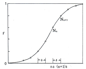
On the other hand, Yamaguchi (1986) pointed out that mapping the solution of a logistic differential equation gives exactly the same value as that of the solution of the original differential equation irrespective of the span of the difference.
Mapping?of?solution?of?logistic?equation
Source: Yamaguchi, 1986.
When N at time nd, N (nd) is expressed by Nn, the mapping of the solution (32’) of the differential equation (31) can be described by (33) and (34):
where,
As shown in Figure 9, the Nn+1 value in (34) always fulfills the solution (32’) of the differential equation irrespective of the size of time span, d. This could be a matter of course but is the same phenomenon observed in that the solution (30’) of difference equations (21), (22), and (23) satisfies the solution (32’’) of the original logistic differential equation (31), the derivation is different though.